用Python实现神经网络(二)
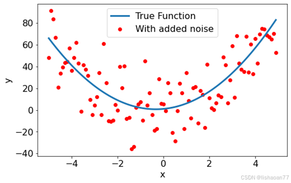
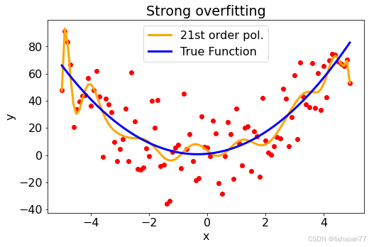
#Overfitting是机器学习的主要问题。下面我们来看一下过拟合现像:
import numpy as np
import matplotlib.pyplot as plt
import matplotlib as mpl
import tensorflow as tf
from scipy.optimize import curve_fit
# Generic matplotlib parameters for plots and figures
mpl.rcParams['figure.figsize'] = [8,5]
font = {'size' : 16}
mpl.rc('font', **font)
def func_0(p, a):
return a
def func_2(p, a, b, c):
return a+b*p + c*p**2
def func_3(p, a, b, c,d):
return a+b*p + c*p**2+d*p**3
def func_5(p, a, b, c,d,e,f):
return a+b*p + c*p**2+d*p**3+e*p**4+f*p**5
def func_14(p, a,b,c,d,e,f,g,h, i,j,k,l,m,n,o):
return a+b*p + c*p**2+d*p**3+e*p**4 + f*p**5 + g*p**6 + h*p**7+i*p**8 + j*p**9+k*p**10+l*p**11 + m*p**12 + n*p**13 + o*p**14
def func_21(p, a,b,c,d,e,f,g,h, i,j,k,l,m,n,o, q, r, s, t, u, v, x):
return a+b*p + c*p**2+d*p**3+e*p**4 + f*p**5 + g*p**6 + h*p**7+i*p**8 + j*p**9+k*p**10+l*p**11 + m*p**12 + n*p**13 + o*p**14+q*p**15+r*p**16+s*p**17+t*p**18+u*p**19+v*p**20+x*p**21
def func_1(p, a, b):
return a+b*p
x = np.arange(-5.0, 5.0, 0.1, dtype = np.float64)
y = func_2(x, 1,2,3)+18.0*np.random.normal(0, 1, size=len(x))
popt, pcov = curve_fit(func_2, x, y)
print(popt)
fig = plt.figure()
ax = fig.add_subplot(1, 1, 1)
ax.scatter(x,y, color = 'red', label = 'With added noise')
ax.plot(x, func_2(x, 1,2,3), lw = 3, label = 'True Function')
ax.set_xlabel('x')
ax.set_ylabel('y')
plt.legend()
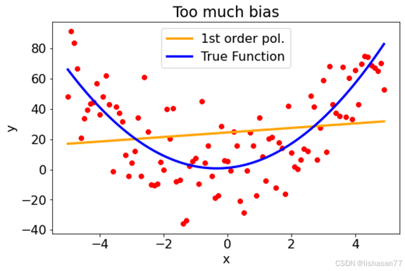
一次多项式
popt, pcov = curve_fit(func_1, x, y)
print(popt)
fig = plt.figure()
ax = fig.add_subplot(1, 1, 1)
ax.scatter(x,y, color = 'red')
ax.plot(x, func_1(x, popt[0], popt[1]), lw=3, color = 'orange', label = '1st order pol.')
ax.plot(x, func_2(x, 1,2,3), lw = 3, color ='blue', label = 'True Function')
ax.set_xlabel('x')
ax.set_ylabel('y')
ax.set_title('Too much bias')
plt.legend()
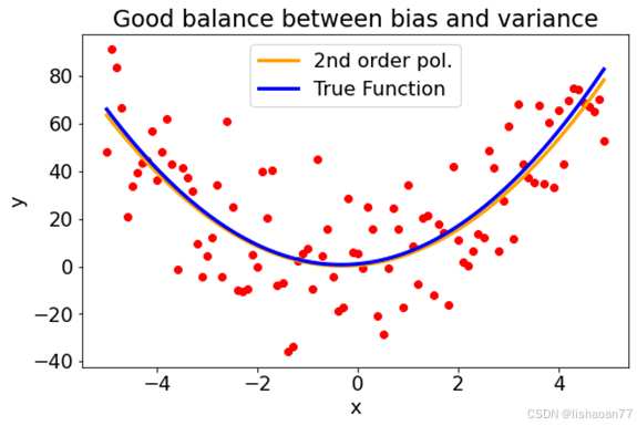
二次多项式
popt, pcov = curve_fit(func_2, x, y)
print(popt)
fig = plt.figure()
ax = fig.add_subplot(1, 1, 1)
ax.scatter(x,y, color = 'red')
ax.plot(x, func_2(x, *popt), lw=3, color ='orange', label = '2nd order pol.')
ax.plot(x, func_2(x, 1,2,3), lw = 3, color ='blue', label = 'True Function')
ax.set_xlabel('x')
ax.set_ylabel('y')
ax.set_title('Good balance between bias and variance')
plt.legend()
21次多项式
popt, pcov = curve_fit(func_21, x, y)
print(popt)
fig = plt.figure()
ax = fig.add_subplot(1, 1, 1)
ax.scatter(x,y, color = 'red')
ax.plot(x, func_21(x, *popt), lw=3,color ='orange', label = '21st order pol.')
ax.plot(x, func_2(x, 1,2,3), lw = 3, color ='blue', label = 'True Function')
ax.set_xlabel('x')
ax.set_ylabel('y')
plt.title('Strong overfitting')
plt.legend()
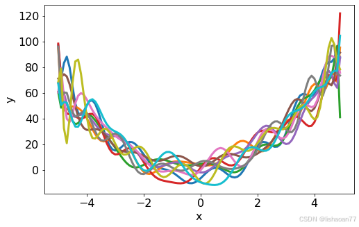
比较蓝线
yy = []
poptl = []
for i in range (0,10):
np.random.seed(seed = i)
yy.append(func_2(x, 1,2,3)+18.0*np.random.normal(0, 1, size=len(x)))
popt, _ = curve_fit(func_21, x, yy[i])
poptl.append(popt)
fig = plt.figure()
ax = fig.add_subplot(1, 1, 1)
for i in range(0,10):
ax.plot(x, func_21(x, *poptl[i]), lw=3)
ax.set_xlabel('x')
ax.set_ylabel('y')
yy = []
poptl = []
for i in range (0,10):
np.random.seed(seed = i)
yy.append(func_2(x, 1,2,3)+18.0*np.random.normal(0, 1, size=len(x)))
popt, _ = curve_fit(func_1, x, yy[i])
poptl.append(popt)
fig = plt.figure()
ax = fig.add_subplot(1, 1, 1)
plt.ylim(0,100)
for i in range(0,10):
ax.plot(x, func_1(x, *poptl[i]), lw=3)
ax.set_xlabel('x')
ax.set_ylabel('y')
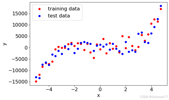
偏置 - 变化的妥协
x = np.arange(-5.0, 5.0, 0.25, dtype = np.float64)
y = func_5(x, 1,2,3,4,5,6)/1.0+2000.0*np.random.normal(0, 1, size=len(x))
ytest = func_5(x, 1,2,3,4,5,6)/1.0+2000.0*np.random.normal(0, 1, size=len(x))
fig = plt.figure()
ax = fig.add_subplot(1, 1, 1)
ax.scatter(x[:,],y[:,], color = 'red', label = 'training data')
ax.scatter(x[:,],ytest[:,], color = 'blue', label = 'test data')
ax.legend();
ax.set_xlabel('x')
ax.set_ylabel('y')
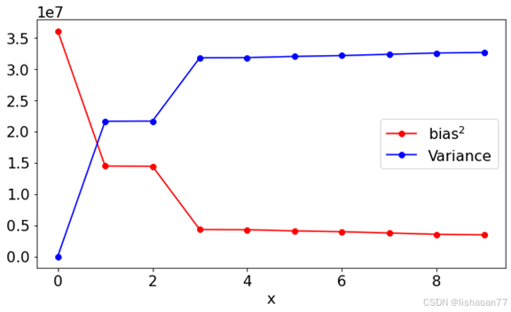
我们来计算偏置和变化用增加复杂度的多项式。我们考虑 0 到10阶, 即常数到 9次多项式(最高次项为 9x9)。
kmax = 10
bias = np.empty(kmax)
variance = np.empty(kmax)
def make_func(N):
def func(x, *p):
res = np.zeros(len(x))
for i in range (0,N+1):
res = res + p[i]*x**i
return res
return func
for K in range (0,kmax):
func = make_func(K)
popt, _ = curve_fit(make_func(K), x, y, p0=[1.0]*(K+1))
bias[K] = np.mean((func(x, *popt)-y)**2)
variance[K] = np.var((func(x, *popt)))
fig = plt.figure()
ax = fig.add_subplot(1, 1, 1)
ax.plot(range(0,kmax),bias, color = 'red', label = r'bias$^2$', marker = 'o')
ax.plot(range(0,kmax),variance, color = 'blue', label = 'Variance', marker = 'o')
ax.set_xlabel('x')
plt.legend()
plt.tight_layout()
神经网络进行回归
xx = x.reshape(len(x),1)
yy = y.reshape(len(y),1)/1000.0+20.0
yytest = ytest.reshape(1,len(ytest))/1000.0+20.0
xx,yy
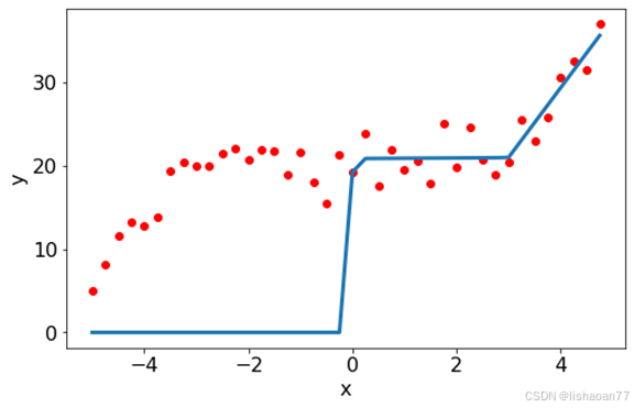
我们尝试一些疯狂的事情:有150个神经元的层。你希望什么?
#tf.reset_default_graph()
input_Dim=1
H1_NN=500
output_Dim=1
np.random.seed(612)
w1=tf.Variable(tf.random.normal([input_Dim, H1_NN], stddev=1))
b1 = tf.Variable(tf.zeros(H1_NN),dtype=tf.float32)
w2=tf.Variable(tf.random.normal([H1_NN,output_Dim], stddev=1))
b2 = tf.Variable(tf.zeros(output_Dim),dtype=tf.float32)
#W=[W1,W2]
#B=[B1,B2]
#定义模型函数
def model(x,w1,b1,w2,b2):
x=tf.matmul(x,w1)+b1
x=tf.nn.relu(x)
x=tf.matmul(x,w2)+b2
pred=tf.nn.relu(x)
return (pred)
#np.random.seed(612)
#W = tf.Variable(np.random.randn(784,10),dtype=tf.float32)
#B = tf.Variable(np.random.randn(10),dtype=tf.float32)
def loss(x,y,w1,b1,w2,b2):
#pred = model(x,w,b)
#loss_=tf.keras.losses.categorical_crossentropy(y_true=y,y_pred=pred)
#Loss_ = 0.5 * tf.reduce_mean(tf.square(Y_train - PRED_train))
#return tf.reduce_mean(loss_)
err = model(x,w1,b1,w2,b2)-y
squared_err = tf.square(err)
return tf.reduce_mean(squared_err)
def grad(x,y,w1,b1,w2,b2):
with tf.GradientTape() as tape:
loss_ = loss(x,y,w1,b1,w2,b2)
return tape.gradient(loss_,[w1,b1,w2,b2])
#def accuracy(x,y,w1,b1,w2,b2):
# pred = model(x,w1,b1,w2,b2)
# correct_prediction=tf.equal(tf.argmax(pred,1),tf.argmax(y,1))
# return tf.reduce_mean(tf.cast(correct_prediction,tf.float32))
cost_history = np.empty(shape=[1], dtype = float)
#learning_rate = tf.placeholder(tf.float32, shape=())
#learning_rate = tf.Variable(tf.random.normal(1))
#设置迭代次数和学习率
#train_epochs = 20
batch_size=1
learning_rate = 0.01
#构建线性函数的斜率和截距
training_epochs=1000
steps=int(training_epochs/batch_size)
loss_list_train = []
loss_list_valid = []
acc_list_train = []
acc_valid_train = []
#training_epochs=100
optimizer= tf.keras.optimizers.Adam(learning_rate=learning_rate)
#开始训练,轮数为epoch,采用SGD随机梯度下降优化方法
for epoch in range(training_epochs):
#for step in range(steps):
#xs=xx[step*batch_size:(step+1)*batch_size]
#ys=yy[step*batch_size:(step+1)*batch_size]
xs=tf.cast(xx,tf.float32)
ys=tf.cast(yy,tf.float32)
#计算损失,并保存本次损失计算结果
grads=grad(xs,ys,w1,b1,w2,b2)
optimizer.apply_gradients(zip(grads,[w1,b1,w2,b2]))
loss_train =loss(xs,ys,w1,b1,w2,b2).numpy()
#loss_valid =loss(valid_x,valid_y,W,B).numpy()
#acc_train=accuracy(xs,ys,w1,b1,w2,b2).numpy()
#acc_valid=accuracy(valid_x,valid_y,W,B).numpy()
loss_list_train.append(loss_train)
#loss_list_valid.append(loss_valid)
#acc_list_train.append(acc_train)
#acc_valid_train.append(acc_valid)
#print("epoch={:3d},train_loss={:.4f},train_acc={:.4f},val_loss={:.4f},val_acc={:.4f}".format(epoch+1,loss_train,acc_train,loss_valid,acc_valid))
if (epoch % 100 == 0):
print("epoch={:3d},train_loss={:.4f}".format(epoch+1,loss_train))
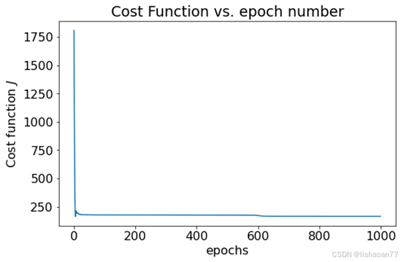
plt.figure()
plt.title("Cost Function vs. epoch number")
plt.xlabel("epochs")
plt.ylabel("Cost function $J$")
plt.plot(range(len(loss_list_train)), loss_list_train)
xs=tf.cast(xx,tf.float32)
ys=tf.cast(yy,tf.float32)
pred_y=model(xs,w1,b1,w2,b2).numpy()
#pred_y.shape
mse=loss(xs,ys,w1,b1,w2,b2).numpy()
#mse = tf.reduce_mean(tf.square(pred_y - yy))
print("MSE: %.4f" % mse)
fig = plt.figure()
ax = fig.add_subplot(1, 1, 1)
ax.scatter(xx[:,0],yy, color = 'red')
ax.plot(xx[:,0], pred_y.flatten(), lw=3)
ax.set_xlabel('x')
ax.set_ylabel('y')