当前位置：首页 > news >正文

[论文精读]Semi-Supervised Classification with Graph Convolutional Networks

news 2025/6/26 11:12:17

论文原文：[1609.02907] Semi-Supervised Classification with Graph Convolutional Networks (arxiv.org)

论文代码：GitHub - tkipf/gcn: Implementation of Graph Convolutional Networks in TensorFlow

英文是纯手打的！论文原文的summarizing and paraphrasing。可能会出现难以避免的拼写错误和语法错误，若有发现欢迎评论指正！文章偏向于笔记，谨慎食用！

1. 省流版

1.1. 心得

（1）怎么开头我就不知道在说什么啊这个论文感觉表述不是很清晰？

（2）数学部分推理很清晰

1.2. 论文框架图

2. 论文逐段阅读

2.1. Abstract

①Their convolution is based on localized first-order approximation

②They encode node features and local graph structure in hidden layers

2.2. Introduction

①The authors think adopting Laplacian regularization in the loss function helps to label:

$\mathcal{L}=\mathcal{L}_0+\lambda\mathcal{L}_{\text{reg}},\quad\\\\\text{with}\quad\mathcal{L}_{\text{reg}}=\sum_{i,j}A_{ij}\|f(X_i)-f(X_j)\|^2=f(X)^\top\Delta f(X)$

where $\mathcal{L}_0$ represents supervised loss with labeled data,

$f\left ( \right )$ is a differentiable function,

$\lambda$ denotes weight,

$X$ denotes matrix with combination of node feature vectors,

$\triangle =D-A$ represents the unnormalized graph Laplacian,

$A$ is adjacency matrix,

$D$ is degree matrix.

②The model trains labeled nodes and is able to learn labeled and unlabeled nodes

③GCN achieves higher accuracy and efficiency than others

2.3. Fast approximate convolutions on graphs

①GCN (undirected graph):

$H^{(l+1)}=\sigma\Big(\tilde{D}^{-\frac{1}{2}}\tilde{A}\tilde{D}^{-\frac{1}{2}}H^{(l)}W^{(l)}\Big)$

where $\tilde{A}$ denotes autoregressive adjacency matrix, which means $\tilde{A}=A+I_{N}$ ,

$I_{N}$ denotes identity matrix,

$\tilde{D}$ denotes autoregressive degree matrix,

$W^{(l)}$ represents the trainable weight matrix in $l$ -th layer,

$H^{(l)}$ denotes the activation matrix in $l$ -th layer,

$\sigma \left ( \right )$ represents activation function

2.3.1. Spectral graph convolutions

①Spectral convolutions on graphs:

$g_{\theta }\star x=Ug_{\theta }U^{T}x$

where the filter $g_{\theta }=diag\left ( \theta \right )$ ,

$U$ comes from normalized graph Laplacian $L=I_{N}-D^{-\frac12}AD^{-\frac12}=U\Lambda U^{T}$ and is the matrix of $L$ 's eigenvectors,

$\Lambda$ denotes a diagonal matrix with eigenvalues.

②However, it is too time-consuming to compute matrix especially for large graph. Ergo, approximating it in $K$ -th order by Chebyshev polynomials:

$g_{\theta^{\prime}}(\Lambda)\approx\sum_{k=0}^K\theta_k^{\prime}T_k(\tilde{\Lambda})$

where $\tilde{\Lambda}=\frac{2}{\lambda_{\max}}\Lambda-I_{N}$ ,

${\theta }'$ denotes Chebyshev coefficients vector,

recursive Chebyshev polynomials are $T_{k}\left ( x \right )=2xT_{k-1}(x)-T_{k-2}(x)$ with baseline $T_{0}(x)=1$ and $T_{1}(x)=x$

③Then get new function:

$g_{\theta'}\star x\approx\sum_{k=0}^{K}\theta'_kT_k(\tilde{L})x$

where $\tilde{L}=\frac{2}{\lambda_{\max}}L-I_{N}$ , $(U\Lambda U^\top)^k=U\Lambda^kU^\top$ .

④Through this approximation method, time complexity reduced from $O\left ( n^{2} \right )$ to $O\left ( E \right )$

2.3.2. Layer-wise linear model

①Then, the authors stack the function above to build multiple conv layers and set $K=1$ , $\lambda _{max}\approx 2$

②They simplified 2.3.1. ③ to:

$g_{\theta'}\star x\approx\theta'_0x+\theta'_1\left(L-I_N\right)x=\theta'_0x-\theta'_1D^{-\frac{1}{2}}AD^{-\frac{1}{2}}x$

where $\theta'_0$ and $\theta'_1$ are free parameters

③Nevertheless, more parameters bring more overfitting problem. It leads the authors change the expression to:

$g_\theta\star x\approx\theta\left(I_N+D^{-\frac{1}{2}}AD^{-\frac{1}{2}}\right)x$

where they define $\theta=\theta_0^{\prime}=-\theta_1^{\prime}$ ,

eigenvalues are in $\left [ 0,2 \right ]$ .

But keep using it may cause exploding/vanishing gradients or numerical instabilities.

④Then they adjust $I_{N}+D^{-\frac{1}{2}}AD^{-\frac{1}{2}}\rightarrow\tilde{D}^{-\frac{1}{2}}\tilde{A}\tilde{D}^{-\frac{1}{2}}$

⑤The convolved signal matrix $\begin{aligned}Z&\in\mathbb{R}^{N\times F}\end{aligned}$ :

$Z=\tilde{D}^{-\frac12}\tilde{A}\tilde{D}^{-\frac12}X\Theta$

where $C$ denotes input channels, namely feature dimensionality of each node,

$F$ denotes the number of filters or feature maps,

$\Theta\in\mathbb{R}^{C\times F}$ represents matrix of filter parameters

2.4. Semi-supervised node classification

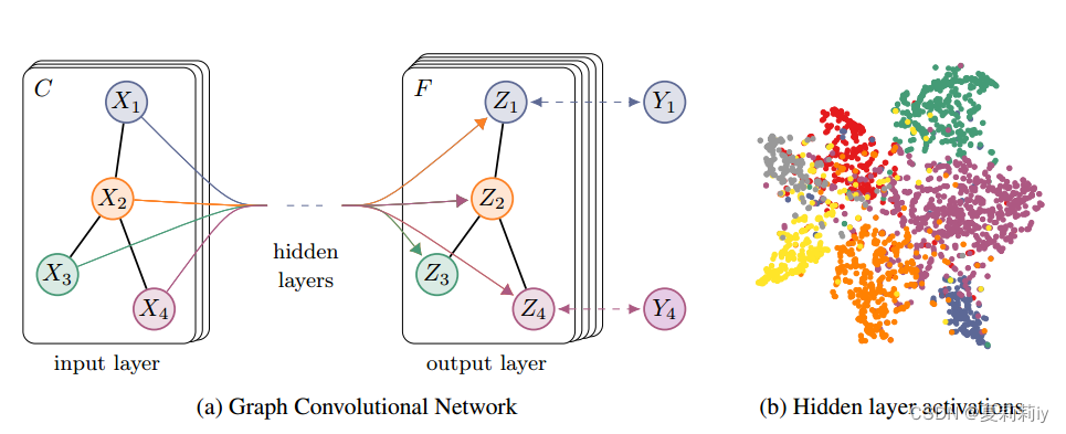
2.4.1. Example

2.4.2. Implementation

2.5. Related work

2.5.1. Graph-based semi-supervised learning

2.5.2. Neural networks on graphs

2.6. Experiments

2.6.1. Datasets

2.6.2. Experimental set-up

2.6.3. Baselines

2.7. Results

2.7.1. Semi-supervised node classifiication

2.7.2. Evaluation of propagation model

2.7.3. Training time per epoch

2.8. Discussion

2.8.1. Semi-supervised model

2.8.2. Limitations and future work

2.9. Conclusion

3. 知识补充

4. Reference List

Kipf, T. & Welling, M. (2017) 'Semi-Supervised Classification with Graph Convolutional Networks', ICLR 2017, doi: https://doi.org/10.48550/arXiv.1609.02907

查看全文

http://www.lryc.cn/news/195282.html