AlexNet训练和测试CIFAR10
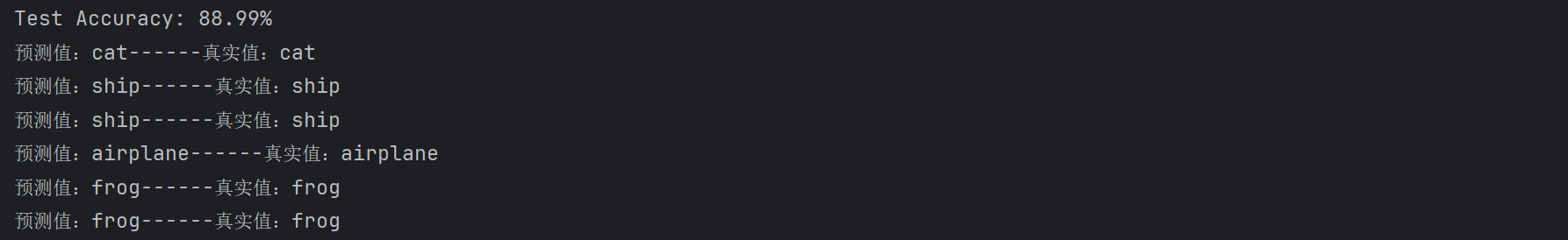
使用AlexNet训练和测试CIFAR10,最终测试精度为88.99%
1.AlexNet模型修改
由于原版的AlexNet网络的输入是3 × 224 × 224,这是当年 ImageNet 比赛的标准输入尺寸,所以原版 AlexNet 第一层卷积核设定为:
nn.Conv2d(3, 64, kernel_size=11, stride=4, padding=2)
而如果是训练CIFAR10( 3 x 32 x 32 ),就要改网络结构以适配小输入
nn.Conv2d(3, 64, kernel_size=3, stride=1, padding=1) # 小卷积核
修改后的模型为:
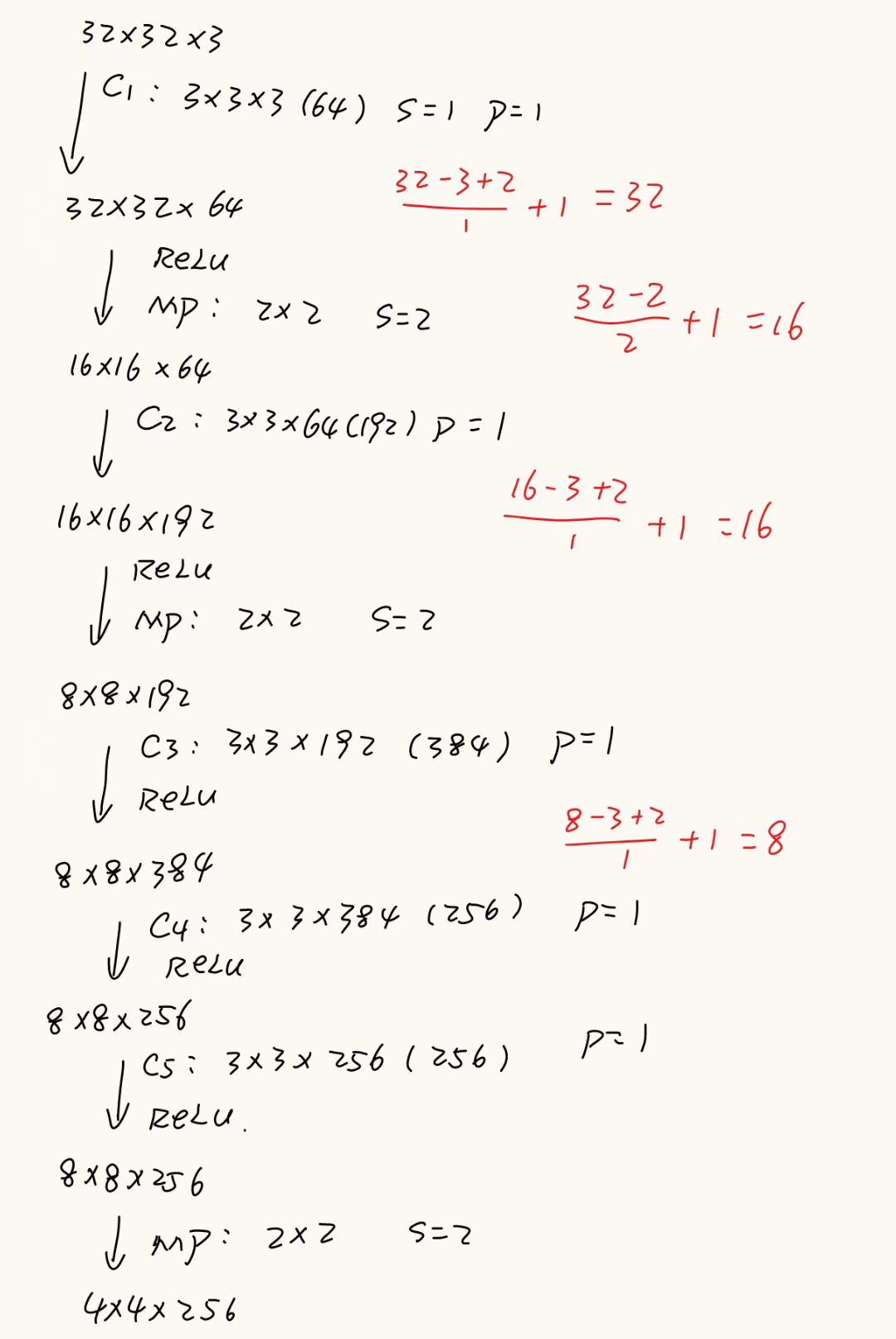
特征提取层代码:
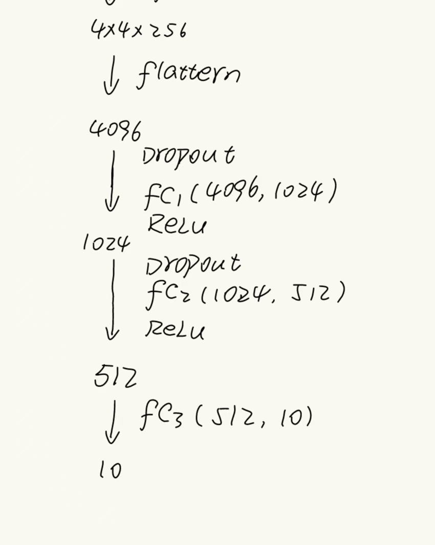
self.features = nn.Sequential(nn.Conv2d(in_channels=3, out_channels=64, kernel_size=3, stride=1, padding=1),nn.ReLU(inplace=True),nn.MaxPool2d(kernel_size=2, stride=2),nn.Conv2d(in_channels=64, out_channels=192, kernel_size=3, stride=1, padding=1),nn.ReLU(inplace=True),nn.MaxPool2d(kernel_size=2, stride=2),nn.Conv2d(in_channels=192, out_channels=384, kernel_size=3, stride=1, padding=1),nn.ReLU(inplace=True),nn.Conv2d(in_channels=384, out_channels=256, kernel_size=3, stride=1, padding=1),nn.ReLU(inplace=True),nn.Conv2d(in_channels=256, out_channels=256, kernel_size=3, stride=1, padding=1),nn.ReLU(inplace=True),nn.MaxPool2d(kernel_size=2, stride=2) #4*4*256)线性分类器代码:
self.classifier = nn.Sequential(nn.Dropout(),nn.Linear(in_features=256 * 4 * 4, out_features=1024),nn.ReLU(inplace=True),nn.Dropout(),nn.Linear(in_features=1024, out_features=512),nn.ReLU(inplace=True),nn.Linear(in_features=512, out_features=10),)前向传播代码:
def forward(self, x):x = self.features(x)x = torch.flatten(x, 1)x = self.classifier(x)return x主函数代码:
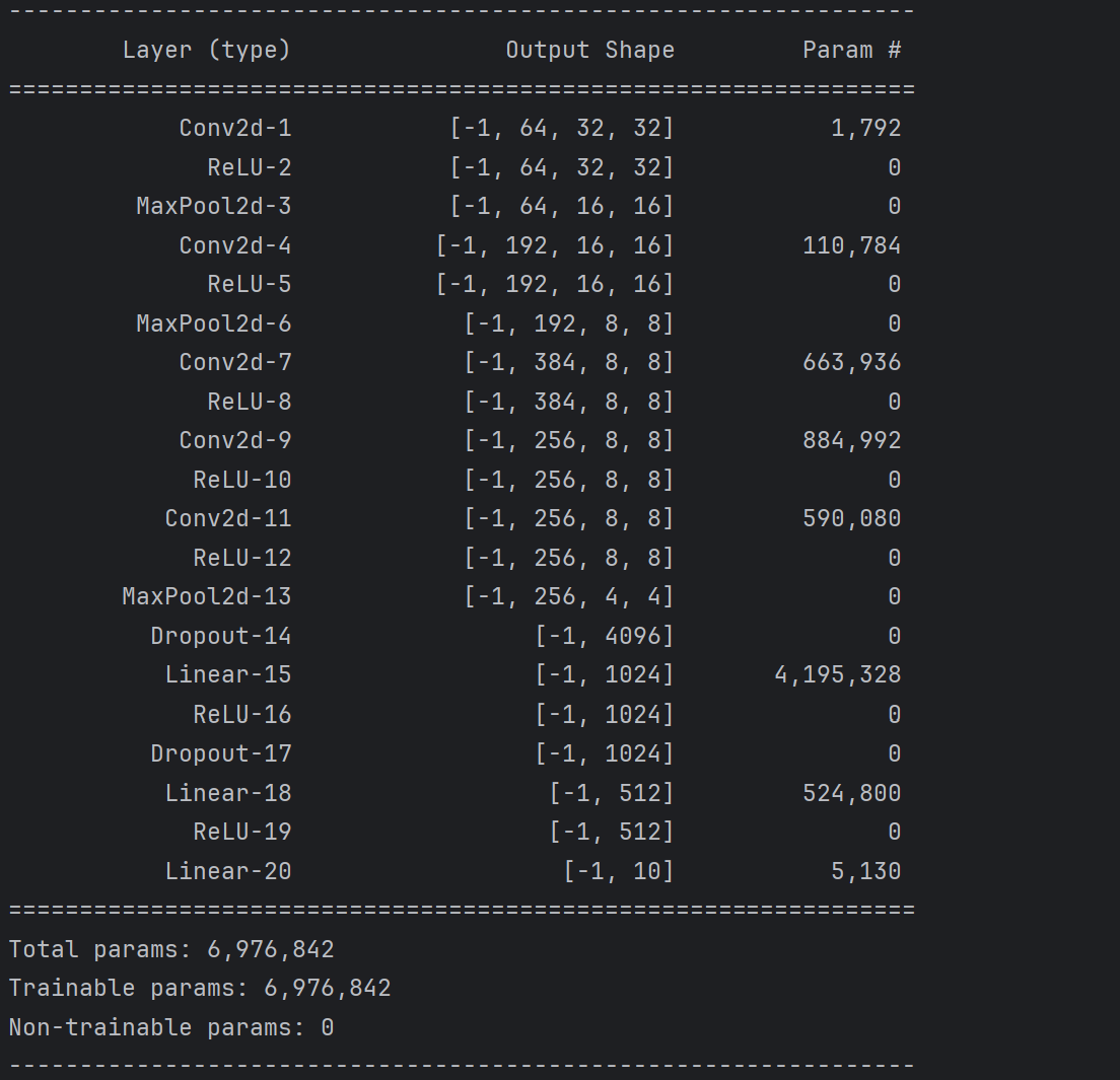
if __name__ == '__main__':device = torch.device("cuda:0" if torch.cuda.is_available() else "cpu")model = AlexNet().to(device)print(summary(model, (3, 32, 32)))最终网络参数图:
2. 模型训练修改
2.1 修改图像预处理的代码
#== 图像预处理,可预防过拟合transform = transforms.Compose([transforms.RandomCrop(32, padding=4),transforms.RandomHorizontalFlip(),transforms.ToTensor(),transforms.Normalize(mean=[0.4914, 0.4822, 0.4465],std=[0.2470, 0.2435, 0.2616]),Cutout(n_holes=1, length=8) #应用Cutout]) 2.2 Cutout 数据增强,是图像级别的正则化
# ===== Cutout 数据增强 =====
class Cutout(object):def __init__(self, n_holes=1, length=8):self.n_holes = n_holesself.length = lengthdef __call__(self, img):h, w = img.size(1), img.size(2)mask = np.ones((h, w), np.float32)for _ in range(self.n_holes):y = np.random.randint(h)x = np.random.randint(w)y1 = np.clip(y - self.length // 2, 0, h)y2 = np.clip(y + self.length // 2, 0, h)x1 = np.clip(x - self.length // 2, 0, w)x2 = np.clip(x + self.length // 2, 0, w)mask[y1:y2, x1:x2] = 0.mask = torch.from_numpy(mask)mask = mask.expand_as(img)img = img * maskreturn img
并且在数据预处理中应用,Cutout(n_holes=1, length=8)
2.3 选择合适的优化器
这里有两种优化器,分别对应不同的应用场景
optimizer = torch.optim.Adam(model.parameters(), lr=0.001)
optimizer = torch.optim.SGD(model.parameters(), lr=0.01, momentum=0.9, weight_decay=5e-4)| 对比项 | Adam | SGD + Momentum |
|---|---|---|
| 学习率调节 | 自适应(每个参数单独调整) | 固定(需手动调整) |
| 超参数敏感性 | 低 | 高 |
| 收敛速度 | 初期快 | 初期慢,但收敛稳定 |
| 最终精度 | 有时略低 | 高(尤其大规模训练) |
| 适用场景 | 小数据集、快速试验、NLP、稀疏梯度 | 大数据集、图像分类、需要高精度的任务 |
| 正则化 | 默认无 weight decay | 常配合 weight decay 防过拟合 |
如果是快速验证模型 → 用
Adam(lr=0.001),调参少,见效快。如果是正式训练大模型(尤其图像分类) → 用
SGD(momentum=0.9, weight_decay=5e-4),配合StepLR或CosineAnnealingLR调度,效果更稳。
这里选用SGD + Momentum
2.4 选择合适的学习率调度器
这里也有两种学习率调度器,分别对应不同的应用场景
scheduler = torch.optim.lr_scheduler.StepLR(optimizer, step_size=30, gamma=0.1)
scheduler = torch.optim.lr_scheduler.CosineAnnealingLR(optimizer, T_max=num_epochs)这两个学习率调度器的降学习率方式完全不同,一个是“阶梯状”,一个是“余弦曲线”
| 特性 | StepLR | CosineAnnealingLR |
|---|---|---|
| 曲线形状 | 阶梯状 | 平滑余弦曲线 |
| 调整频率 | 固定间隔突变 | 每个 epoch 都变 |
| 超参数 | step_size, gamma | T_max(+ 可选 eta_min) |
| 稳定性 | 突然变小,可能不稳定 | 平滑,训练更稳定 |
| 适用场景 | 分阶段收敛的任务 | 精细调控,避免学习率突变 |
如果你是 ImageNet / CIFAR-10 + SGD → 常用
CosineAnnealingLR,稳定收敛。如果你的任务 loss 分阶段下降明显 → 用
StepLR,降到下一个“训练阶段”。
这里选用CosineAnnealingLR学习率调度器
注意:在 epoch 循环末尾加入scheduler.step()
for epoch in range(num_epochs):train_one_epoch(...)validate(...)scheduler.step() # 每个 epoch 结束后调用
完整训练代码
import torch #pytorch基础库
from torchvision.datasets import CIFAR10 #导入FashionMNIST数据集
from torchvision import transforms #数据处理库
import torch.utils.data as data #数据处理库
import torch.nn as nn #pytorch中线性库
import matplotlib.pyplot as plt #可视化库
from model import AlexNet #从前面的model文件中导入LeNet网络结构import copy
import time
import pandas as pd
import numpy as np
# ===== Cutout 数据增强 =====
class Cutout(object):def __init__(self, n_holes=1, length=8):self.n_holes = n_holesself.length = lengthdef __call__(self, img):h, w = img.size(1), img.size(2)mask = np.ones((h, w), np.float32)for _ in range(self.n_holes):y = np.random.randint(h)x = np.random.randint(w)y1 = np.clip(y - self.length // 2, 0, h)y2 = np.clip(y + self.length // 2, 0, h)x1 = np.clip(x - self.length // 2, 0, w)x2 = np.clip(x + self.length // 2, 0, w)mask[y1:y2, x1:x2] = 0.mask = torch.from_numpy(mask)mask = mask.expand_as(img)img = img * maskreturn img
#===数据加载函数
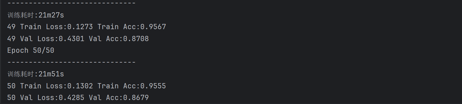
def train_val_process():#== 图像预处理,可预防过拟合transform = transforms.Compose([transforms.RandomCrop(32, padding=4),transforms.RandomHorizontalFlip(),transforms.ToTensor(),transforms.Normalize(mean=[0.4914, 0.4822, 0.4465],std=[0.2470, 0.2435, 0.2616]),Cutout(n_holes=1, length=8)])#== 下载数据集train_data = CIFAR10(root='./data',train=True,transform=transform,download=True)#== 划分数据集 80%为训练集,20%为验证集train_data,val_data =data.random_split(train_data,[round(len(train_data)*0.8),round(len(train_data)*0.2)])#== 加载训练集和验证集train_loader = data.DataLoader(train_data,batch_size=64,shuffle=True,num_workers=4)val_loader = data.DataLoader(val_data,batch_size=64,shuffle=False,num_workers=4)return train_loader,val_loaderdef model_train_process(model, train_loader, val_loader, num_epochs):# 如果有GPU用GPU,没有GPU用CPUdevice = torch.device("cuda:0" if torch.cuda.is_available() else "cpu")# 优化器#optimizer = torch.optim.Adam(model.parameters(), lr=0.001)optimizer = torch.optim.SGD(model.parameters(), lr=0.01, momentum=0.9, weight_decay=5e-4)#scheduler = torch.optim.lr_scheduler.StepLR(optimizer, step_size=30, gamma=0.1)scheduler = torch.optim.lr_scheduler.CosineAnnealingLR(optimizer, T_max=num_epochs)# loss函数使用交叉熵loss,来更新模型参数# 回归一般用均方差,分类一般用交叉熵criterion = nn.CrossEntropyLoss()# 将模型放入设备model = model.to(device)# 复制当前模型参数,以便找到最优模型参数# 这里要导入包,import copybest_model_wts = copy.deepcopy(model.state_dict())# 参数初始化# 最优精度best_acc = 0.0# train集loss列表train_loss_all = []# val集loss列表val_loss_all = []# train集val列表train_acc_all = []# val集val列表val_acc_all = []# 保存当前时间,以便计算训练用时# 导包 import timesince = time.time()# 轮次循环for epoch in range(num_epochs):print('Epoch {}/{}'.format(epoch + 1, num_epochs))print('-' * 30)# 轮次初始化train_loss = 0.0val_loss = 0.0train_acc = 0.0val_acc = 0.0train_num = 0.0 # 训练样本数val_num = 0.0 # 验证样本数# 开启训练模式model.train()# batch循环# 每一轮中从train_loader中按batch中取出标签和特征for batch_idx, (inputs, targets) in enumerate(train_loader):# 将特征放入设备中inputs, targets = inputs.to(device), targets.to(device)# 前向传播outputs = model(inputs)# 经过softmax得到batch中最大值对应的行标pred = torch.argmax(outputs, dim=1)# 计算每一batch的lossloss = criterion(outputs, targets)# 梯度置为0,开始反向传播optimizer.zero_grad()# 反向传播loss.backward()# 更新网络参数optimizer.step()# 计算该batch的训练集的loss# input.size(0)为数据集大小train_loss += loss.item() * inputs.size(0)#计算训练集的准确度train_acc += torch.sum(pred == targets).item()# 计算训练集样本数train_num += inputs.size(0)model.eval()with torch.no_grad():for batch_idx, (inputs, targets) in enumerate(val_loader):inputs, targets = inputs.to(device), targets.to(device)outputs = model(inputs)pred = torch.argmax(outputs, dim=1)loss = criterion(outputs, targets)val_loss += loss.item() * inputs.size(0)val_acc += torch.sum(pred == targets).item()val_num += inputs.size(0)scheduler.step()# 计算用时并且打印输出time_use = time.time() - sinceprint("训练耗时:{:.0f}m{:.0f}s".format(time_use // 60, time_use % 60))# 计算并且保存每一轮次的loss和准确度并且打印输出time_use = time.time() - since# 计算并且保存每一次迭代的loss和准确度train_loss_all.append(train_loss / train_num)val_loss_all.append(val_loss / val_num)train_acc_all.append(train_acc / train_num)val_acc_all.append(val_acc / val_num)print("{} Train Loss:{:.4f} Train Acc:{:.4f}".format(epoch + 1, train_loss_all[-1], train_acc_all[-1]))print("{} Val Loss:{:.4f} Val Acc:{:.4f}".format(epoch + 1, val_loss_all[-1], val_acc_all[-1]))# 寻找最高准确度的权重if val_acc_all[-1] > best_acc:#保存当前的最高准确度best_acc = val_acc_all[-1]# 保存当前的参数best_model_wts = copy.deepcopy(model.state_dict())# 加载最优模型model.load_state_dict(best_model_wts)# 保存最优模型torch.save(model.state_dict(), './model.pth')train_process = pd.DataFrame(data={"epoch": range(1, num_epochs + 1),"train_loss_all": train_loss_all,"train_acc_all": train_acc_all,"val_loss_all": val_loss_all,"val_acc_all": val_acc_all})return train_processdef plot(train_process):#图的大小12*4plt.figure(figsize=(12,4))#将图分为一行两列,并且现在这个图为1plt.subplot(121)plt.plot(train_process['epoch'],train_process.train_loss_all,'-ro',label='train_loss')plt.plot(train_process['epoch'],train_process.val_loss_all,'-bs',label='val_loss')plt.legend()plt.xlabel('epoch')plt.ylabel('loss')plt.subplot(122)plt.plot(train_process['epoch'],train_process.train_acc_all,'-ro',label='train_acc')plt.plot(train_process['epoch'],train_process.val_acc_all,'-bs',label='val_acc')plt.legend()plt.xlabel('epoch')plt.ylabel('accuracy')plt.show()if __name__ == '__main__':model = AlexNet()train_loader,val_loader = train_val_process()train_process = model_train_process(model,train_loader,val_loader,num_epochs=50)plot(train_process)
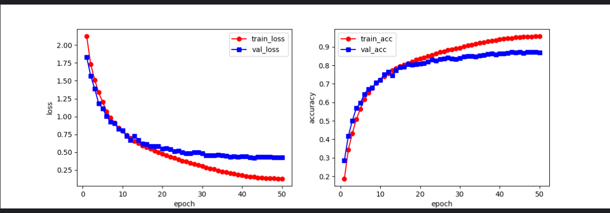
训练结果:
3. 测试代码:
import torch
from torch.utils.data import DataLoader
from torchvision import transforms
from torchvision.datasets import CIFAR10
from model import AlexNetdef test_data_loader():transform = transforms.Compose([transforms.ToTensor(),transforms.Normalize(mean=[0.4914, 0.4822, 0.4465],std=[0.2470, 0.2435, 0.2616])])test_data = CIFAR10(root='./data', train=False, transform=transform)test_loader = DataLoader(test_data, batch_size=1, shuffle=False)return test_loaderdef test_model():device = torch.device('cuda' if torch.cuda.is_available() else 'cpu')model.to(device)model.eval()test_corrects = 0total = 0with torch.no_grad():for inputs,labels in test_data_loader():inputs = inputs.to(device)labels = labels.to(device)outputs = model(inputs)preds = torch.argmax(outputs, dim=1)test_corrects += torch.sum(preds == labels).item()total += labels.size(0)test_acc = test_corrects / totalprint(f'Test Accuracy: {test_acc * 100:.2f}%')return test_accdef predict(model,test_loader):device = torch.device('cuda' if torch.cuda.is_available() else 'cpu')model = model.to(device)model.eval()classes = ['airplane', 'automobile', 'bird', 'cat', 'deer', 'dog', 'frog', 'horse', 'ship', 'truck']with torch.no_grad():for inputs,labels in test_loader:inputs = inputs.to(device)labels = labels.to(device)outputs = model(inputs)preds = torch.argmax(outputs, dim=1)pred_labels = preds.item()true_labels = labels.item()print(f"预测值:{classes[pred_labels]}------真实值:{classes[true_labels]}")if __name__ == '__main__':model = AlexNet()model.load_state_dict(torch.load('./model.pth'))test_loader = test_data_loader()test_acc = test_model()predict(model,test_loader)
测试结果: