深入解析RNN神经网络原理与应用
循环神经网络
RNN神经网络
序列模型
通常在自然语言,音频,视频以及其他序列数据的模型
类型
-
语音识别:输入一段文字输出对应的文字

-
情感分类:输入一段表示用户情感的文字,输出情感类别或者评分

-
机器翻译:两种语言互译

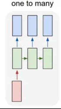
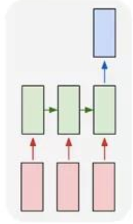
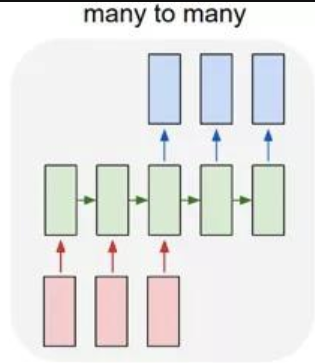
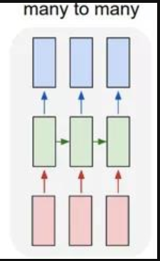
架构类型
-
一对一:一个输入(单一标签)对应一个输出(单一标签)

-
一对多:一个输入对应多个输出;多用于图片的对象识别,比如输入一张图片,输出一段文本序列
-
多对一:多个输入对应一个输出,多用于文本分类或视频分类,即输入一段文本或视频片段,输出类别
-
多对多(1):常用于机器翻译
-
多对多(2):广泛用于序列标注
基本结构
与全连接神经网络和卷积神经网络不同的是:
- RNN神经网络输入特征是有时序的,而前面我们所学习的神经网络输入特征都是同时输入的
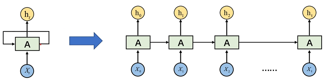
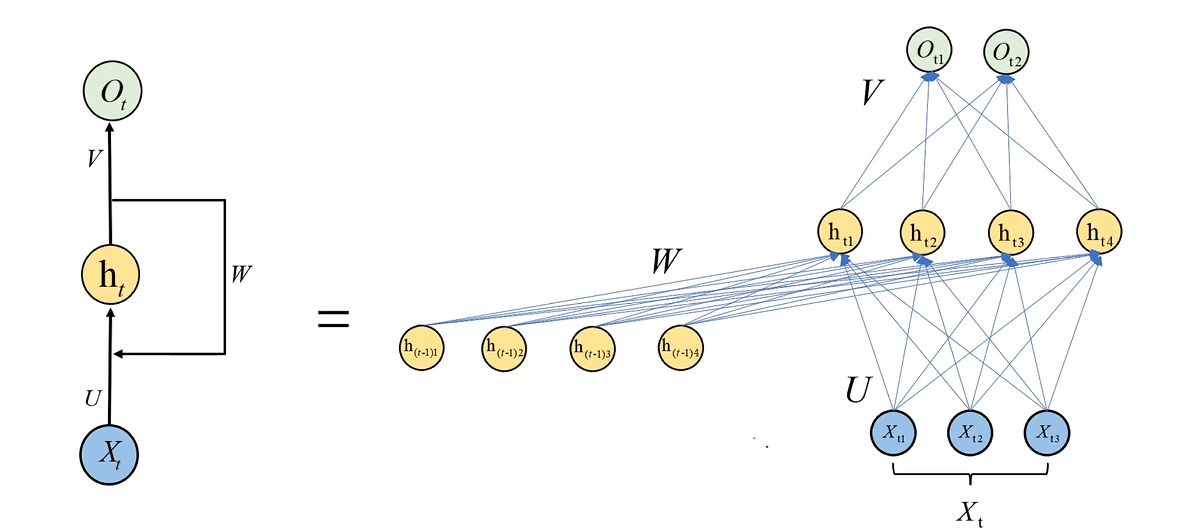
右图是左图的展开形式A为计算单元,类似于隐藏层Xt表示t时刻的输入特征向量,Xt=(Xt1,xt2,…,Xt,k)ht表示Xt对应的隐藏层输出
右图是左图的展开形式\\
A为计算单元,类似于隐藏层\\
X_t表示t时刻的输入特征向量,X_t=(X_{t1},x_{t2},\dots,X_{t,k})\\
h_t表示X_t对应的隐藏层输出\\
右图是左图的展开形式A为计算单元,类似于隐藏层Xt表示t时刻的输入特征向量,Xt=(Xt1,xt2,…,Xt,k)ht表示Xt对应的隐藏层输出
怎么理解图中展示的过程?
X0经过计算单元得到隐藏层输出h0,h0与X1一起作为输入,经计算单元得到h1,如此循环;最终的输出ht会包含前面所有输出h0-(t-1)的有用信息
是一个串行而不是并行的过程
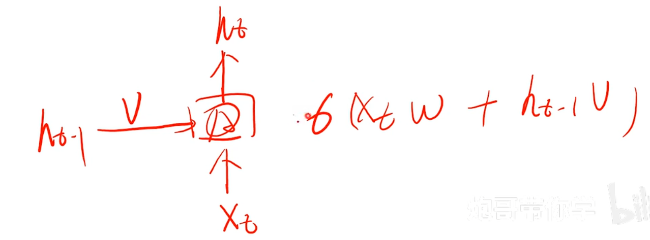
h(t)=activate(Xtw+ht−1v)v:ht−1对应的权重w:Xt对应的权重
h(t)=activate(X_tw+h_{t-1}v)\\
v:h_{t-1}对应的权重\\
w:X_t对应的权重
h(t)=activate(Xtw+ht−1v)v:ht−1对应的权重w:Xt对应的权重
正因为循环神经网络的输入包含前面单元的输出信息,所以它能够学习到时间顺序信息
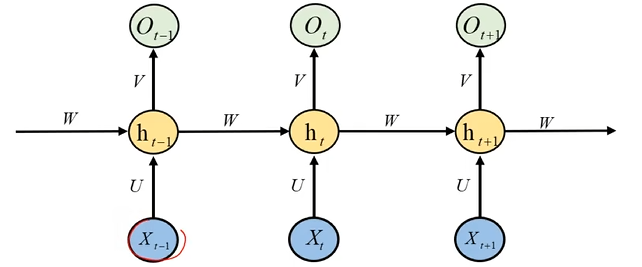
与全连接神经网络的区别
Xt:t时刻的输入特征向量ht:t时刻时隐藏层输出向量Ot:最终的输出层输出向量U,V,W:权重参数
X_t:t时刻的输入特征向量\\
h_t:t时刻时隐藏层输出向量\\
O_t:最终的输出层输出向量\\
U,V,W:权重参数
Xt:t时刻的输入特征向量ht:t时刻时隐藏层输出向量Ot:最终的输出层输出向量U,V,W:权重参数
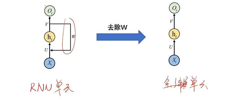
RNN:ht=activate(XtU+ht−1W)全连接神经网络:ht=activate(XtU)
RNN:h_t=activate(X_tU+h_{t-1}W)\\
全连接神经网络:h_t = activate(X_tU)
RNN:ht=activate(XtU+ht−1W)全连接神经网络:ht=activate(XtU)
对于全连接神经网络结构应该这样去展开:
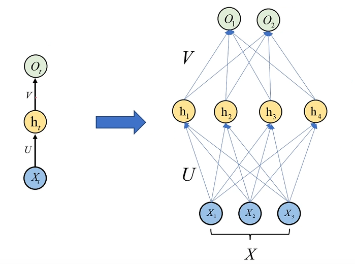
对于RNN神经网络结构应该这样去展开:
全连接神经网络并不把前一时刻的输出当作隐藏层的输入,因此它难以学习到时间序列信息,换句话说,就是全连接神经网络不具有记忆能力
数学模型以及权重共享
Xt:t时刻的输入特征向量ht:t时刻时隐藏层及其输出向量Ot:最终的输出层及其输出向量f():隐藏层激活函数g():输出层激活函数U,V,W:权重参数ht=f(U⋅Xt+W⋅ht−1)Ot=g(V⋅ht)
X_t:t时刻的输入特征向量\\
h_t:t时刻时隐藏层及其输出向量\\
O_t:最终的输出层及其输出向量\\
f():隐藏层激活函数\\
g():输出层激活函数\\
U,V,W:权重参数\\
h_t=f(U\cdot X_t+W\cdot h_{t-1})\\
O_t = g(V\cdot h_t )\\
Xt:t时刻的输入特征向量ht:t时刻时隐藏层及其输出向量Ot:最终的输出层及其输出向量f():隐藏层激活函数g():输出层激活函数U,V,W:权重参数ht=f(U⋅Xt+W⋅ht−1)Ot=g(V⋅ht)
为什么所有的权重参数都不带有时间下标t呢?
和卷积神经网络一样,RNN神经网络也使用了权重共享
为什么
如果每个时刻都训练一套权重,那么权重就太多了
- 权重多,模型复杂,就很容易过拟合
- 权重多也会带来计算量大的问题
词的表示
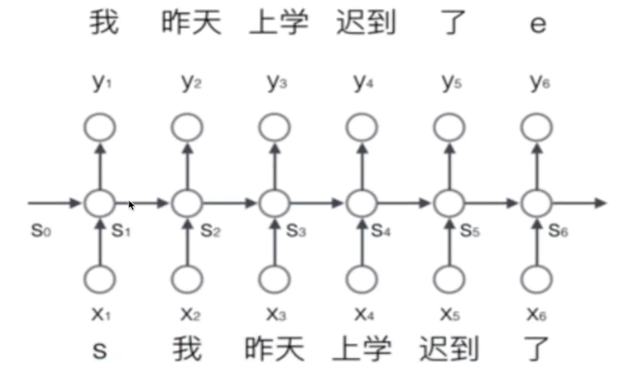
通常对于整个序列,给定一个开始标志s和结束标志e
比如对于句子:我昨天上学迟到了
处理成: s 我 昨天 上学 迟到 了 e
输入到网络中就是一个个分词结果
而为了能够让整个网络能够理解我们的输入(各种语言),我们需要将词用向量表示
-
建立一个包含所有N个序列词的词典包含(开始和结束的两个特殊标志词,以及没有出现过的词等),每个词都有一个唯一索引
-
那么对于每个词,就可以用一个长度为N的向量,使用one-hot编码进行表示
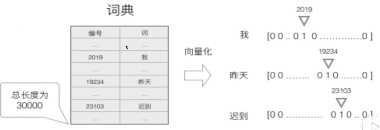
我们就得到了一个高维(维度为N),稀疏(一个1,N-1个0)的向量
输出表示
使用SoftMax;每个时刻的输出是所有词的概率组成的向量
向量化运算
假设输入序列长度为m,神经元个数为n(也可以说是输出维度 )
ht=Tanh(UXt+Wht−1)Ot=SoftMax(Vht)
h_t = Tanh(UX_t+Wh_{t-1})\\
O_t = SoftMax(Vh_t)\\
ht=Tanh(UXt+Wht−1)Ot=SoftMax(Vht)
对于1式
ht=Tanh([h1th2t⋮hnt]n×1=[u11,u12,⋯ ,u1mu21,u22,⋯ ,u2m⋮un1,un2,⋯ ,unm]n×m[x1tx2t⋮xmt]m×1+[w11,w12,⋯ ,w1nw21,w22,⋯ ,w2n⋮wn1,wn2,⋯ ,wnn]n×n[h1t−1h2t−1⋮hnt−1]n×1)(n,1)=(n,m)⋅(m,1)+(n,n)⋅(n,1)
h_t = Tanh(\begin{bmatrix}
h_1^t\\
h_2^t\\
\vdots\\
h_n^t\\
\end{bmatrix}_{n\times 1}=\begin{bmatrix}
u_{11},u_{12},\cdots,u_{1m}\\
u_{21},u_{22},\cdots,u_{2m}\\
\vdots\\
u_{n1},u_{n2},\cdots,u_{nm}
\end{bmatrix}_{n \times m}\begin{bmatrix}
x_1^t\\
x_2^t\\
\vdots\\
x_m^t\\
\end{bmatrix}_{m\times 1}+\begin{bmatrix}
w_{11},w_{12},\cdots,w_{1n}\\
w_{21},w_{22},\cdots,w_{2n}\\
\vdots\\
w_{n1},w_{n2},\cdots,w_{nn}
\end{bmatrix}_{n \times n}\begin{bmatrix}
h_1^{t-1}\\
h_2^{t-1}\\
\vdots\\
h_n^{t-1}\\
\end{bmatrix}_{n\times 1}
)\\
(n,1) = (n,m)\cdot(m,1)+(n,n)\cdot(n,1)
ht=Tanh(h1th2t⋮hntn×1=u11,u12,⋯,u1mu21,u22,⋯,u2m⋮un1,un2,⋯,unmn×mx1tx2t⋮xmtm×1+w11,w12,⋯,w1nw21,w22,⋯,w2n⋮wn1,wn2,⋯,wnnn×nh1t−1h2t−1⋮hnt−1n×1)(n,1)=(n,m)⋅(m,1)+(n,n)⋅(n,1)
可以简化为[U,W][Xtht−1]=(n,n+m)(n+m,1)=(n,1) 可以简化为[U,W][\frac{X_t}{h_{t-1}}]=(n, n+m)(n+m,1) = (n,1) 可以简化为[U,W][ht−1Xt]=(n,n+m)(n+m,1)=(n,1)
对于2式
Ot=SoftMax([v11,v12,⋯ ,v1nv21,v22,⋯ ,v2n⋮vm1,um2,⋯ ,vmn]m×n[h1th2t⋮hnt]n×1)
O_t = SoftMax(\begin{bmatrix}
v_{11},v_{12},\cdots,v_{1n}\\
v_{21},v_{22},\cdots,v_{2n}\\
\vdots\\
v_{m1},u_{m2},\cdots,v_{mn}
\end{bmatrix}_{m \times n}\begin{bmatrix}
h_1^t\\
h_2^t\\
\vdots\\
h_n^t\\
\end{bmatrix}_{n\times 1})
Ot=SoftMax(v11,v12,⋯,v1nv21,v22,⋯,v2n⋮vm1,um2,⋯,vmnm×nh1th2t⋮hntn×1)
Ot是所有m个词的概率向量
前向传播
RNN的前向传播过程事实上就是前面提到的隐藏层计算公式和输出层计算公式
d:输入维度h:隐藏层神经元数
d:输入维度\\
h:隐藏层神经元数
d:输入维度h:隐藏层神经元数
Xt∈R1×dU∈Rh×dW∈Rh×h下面是向量化形式的公式ht=f(U⋅Xt+W⋅ht−1)Ot=g(V⋅ht)
X_t \in R^{1\times d}\\
U \in R^{h\times d}\\
W \in R^{h \times h}\\
下面是向量化形式的公式\\
h_t=f(U\cdot X_t+W\cdot h_{t-1})\\
O_t = g(V\cdot h_t )\\
Xt∈R1×dU∈Rh×dW∈Rh×h下面是向量化形式的公式ht=f(U⋅Xt+W⋅ht−1)Ot=g(V⋅ht)
用一个案例来演示
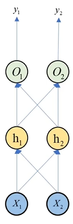
如图所示是RNN中一个时刻t下的单元结构,输入数据含有三个时间步,每个时间步特征向量Xt含有两个元素X1,X2,隐藏层中有2个神经元h1,h2,输出层也有两个神经元O1,O2,最终输出向量含有两个元素y1,y2
Xt=((1,1),(1,1),(2,2))为了方便,我们设定W=V=U=((1,1),(1,1)),所有的激活函数都是不带偏置的线性函数
X_t = ((1,1),(1,1),(2,2))\\
为了方便,我们设定W=V=U=((1,1),(1,1)),所有的激活函数都是不带偏置的线性函数
Xt=((1,1),(1,1),(2,2))为了方便,我们设定W=V=U=((1,1),(1,1)),所有的激活函数都是不带偏置的线性函数
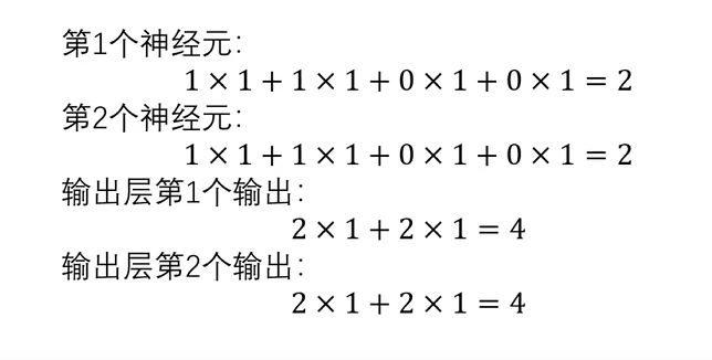
当t=1时X1=(1,1)对于ht1,ht2来说,没有前一个隐藏层的输出值作为输入,因此我们设置h0=(0,0)ht1=f(U1X1+W1h01)=1×1+1×1+1×0+1×0=2ht2=f(U2X1+W2h02)=1×1+1×1+1×0+1×0=2ht=(2,2)Ot1=g(V1ht)=2×1+2×1=4Ot2=g(V2ht)=2×1+2×1=4Ot=(2,2)
当t=1时\\
X_1=(1,1)\\
对于h_{t1},h_{t2}来说,没有前一个隐藏层的输出值作为输入,因此我们设置h_0=(0,0)\\
h_{t1} = f(U_1X_1+W_1h_{01}) = 1\times1+1\times1+1\times0+1\times0=2\\
h_{t2} = f(U_2X_1+W_2h_{02}) = 1\times1+1\times1+1\times0+1\times0=2\\
h_t=(2,2)\\
O_{t1} = g(V_1h_t) = 2\times1+2\times1=4\\
O_{t2} = g(V_2h_t) = 2\times1+2\times1=4\\
O_{t} = (2,2)\\
当t=1时X1=(1,1)对于ht1,ht2来说,没有前一个隐藏层的输出值作为输入,因此我们设置h0=(0,0)ht1=f(U1X1+W1h01)=1×1+1×1+1×0+1×0=2ht2=f(U2X1+W2h02)=1×1+1×1+1×0+1×0=2ht=(2,2)Ot1=g(V1ht)=2×1+2×1=4Ot2=g(V2ht)=2×1+2×1=4Ot=(2,2)
当t=2时h1=(2,2),X2=(1,1)h21=f(U1X2+W1h11)=1×1+1×1+1×2+1×2=6h22=f(U2X2+W1h12)=1×1+1×1+1×2+1×2=6h2=(6,6)O21=g(V1h2)=6×1+6×1=12O22=g(V2h2)=6×1+6×1=12O2=(12,12)
当t=2时\\
h_1=(2,2),X_2=(1,1)\\
h_{21}=f(U_1X_2+W_1h_{11}) = 1\times1+1\times1+1\times2+1\times2=6\\
h_{22}=f(U_2X_2+W_1h_{12}) = 1\times1+1\times1+1\times2+1\times2=6\\
h_2 = (6,6)\\
O_{21}=g(V_1h_2) = 6 \times 1+6\times 1 = 12\\
O_{22}=g(V_2h_2)= 6 \times 1+6\times 1 = 12 \\
O_2 = (12,12)
当t=2时h1=(2,2),X2=(1,1)h21=f(U1X2+W1h11)=1×1+1×1+1×2+1×2=6h22=f(U2X2+W1h12)=1×1+1×1+1×2+1×2=6h2=(6,6)O21=g(V1h2)=6×1+6×1=12O22=g(V2h2)=6×1+6×1=12O2=(12,12)
当t=3时h2=(6,6),X3=(2,2)h31=f(U1X3+W1h21)=1×2+1×2+1×6+1×6=16h32=f(U2X3+W1h22)=1×2+1×2+1×6+1×6=16h3=(16,16)O31=g(V1h31)=1×16+1×16=32O32=g(V2h32)=1×16+1×16=32O3=(32,32) 当t=3时\\ h_2=(6,6),X_3=(2,2)\\ h_{31}=f(U_1X_3+W_1h_{21}) = 1\times2+1\times2+1\times6+1\times6=16\\ h_{32}=f(U_2X_3+W_1h_{22}) = 1\times2+1\times2+1\times6+1\times6=16\\ h_3=(16,16)\\ O_{31}=g(V_1h_{31}) = 1 \times 16+1\times 16 = 32\\ O_{32}= g(V_2h_{32})=1 \times 16+1\times 16 = 32 \\ O_3 = (32,32) 当t=3时h2=(6,6),X3=(2,2)h31=f(U1X3+W1h21)=1×2+1×2+1×6+1×6=16h32=f(U2X3+W1h22)=1×2+1×2+1×6+1×6=16h3=(16,16)O31=g(V1h31)=1×16+1×16=32O32=g(V2h32)=1×16+1×16=32O3=(32,32)
前面所有时间步的信息对后面时间步会有影响,通过反向传播训练W,U,V来控制前面时间步信息的占比
激活函数
RNN通常使用Tanh(双曲正切函数)作为激活函数
Tanh:y=ez−e−zez+e−zy′=1−y2
Tanh:
y = \frac{e^z-e^{-z}}{e^z+e^{-z}} \\
y' = 1 - y^2
Tanh:y=ez+e−zez−e−zy′=1−y2
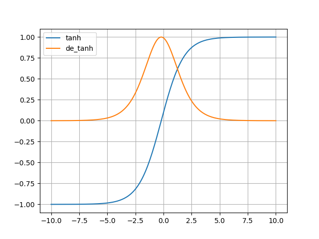
为什么全连接神经网络,卷积神经网络喜欢使用ReLU作为激活函数,而RNN使用Tanh(?)
对于全连接神经网络和CNN:ReLU的导数值只有0或1,Tanh或sigmoid在两级处的导数值都趋近于0,不利于梯度下降
对于RNN:
- RNN与CNN最大的不同就在于会将前一个时刻的隐藏层输出作为此时刻隐藏层的输入;而ReLU的值域在[0,+∞),会导致输出值太大,传递过程中难以控制,出现爆炸;Tanh的值域为[-1,1],在传输隐藏状态ht时,有助于控制其大小
- Tanh关于y轴对称,有助于信息在多个时间步之间稳定传递
交叉熵损失
总损失定义:一整个序列(一个句子)作为训练实例,总误差就是各个时刻的误差之和
Et(yt,yt^)=−ytlog(yt^)E(y,y^)=∑tEt(yt,yt^)=−∑tytlog(yt^)yt:t时刻的正确的词的one−hot编码值yt^:预测的词概率
E_t(y_t,\hat{y_t})=-y_tlog(\hat{y_t})\\
E(y,\hat{y})=\sum_{t}E_t(y_t,\hat{y_t})=-\sum_{t}y_tlog(\hat{y_t})\\
y_t:t时刻的正确的词的one-hot编码值
\\\hat{y_t}:预测的词概率
Et(yt,yt^)=−ytlog(yt^)E(y,y^)=t∑Et(yt,yt^)=−t∑ytlog(yt^)yt:t时刻的正确的词的one−hot编码值yt^:预测的词概率
时间反向传播BPTT
RNN神经网络中反向传播算法利用的是时间反向传播算法BPTT;需要求解所有时间步的梯度之后,利用多变量链式求导法则求解梯度
由于RNN的权重共享以及分时间步计算,总的梯度是各个时间步梯度的加和
- 我们的目标是计算损失关于参数U,V,W,偏置bx,by的梯度
前向传播公式:
ht=Tanh(UXt+Wht−1+bx)Ot=SoftMax(Vht+by)
h_t = Tanh(UX_t+Wh_{t-1}+b_x)\\
O_t = SoftMax(Vh_t+b_y)
ht=Tanh(UXt+Wht−1+bx)Ot=SoftMax(Vht+by)
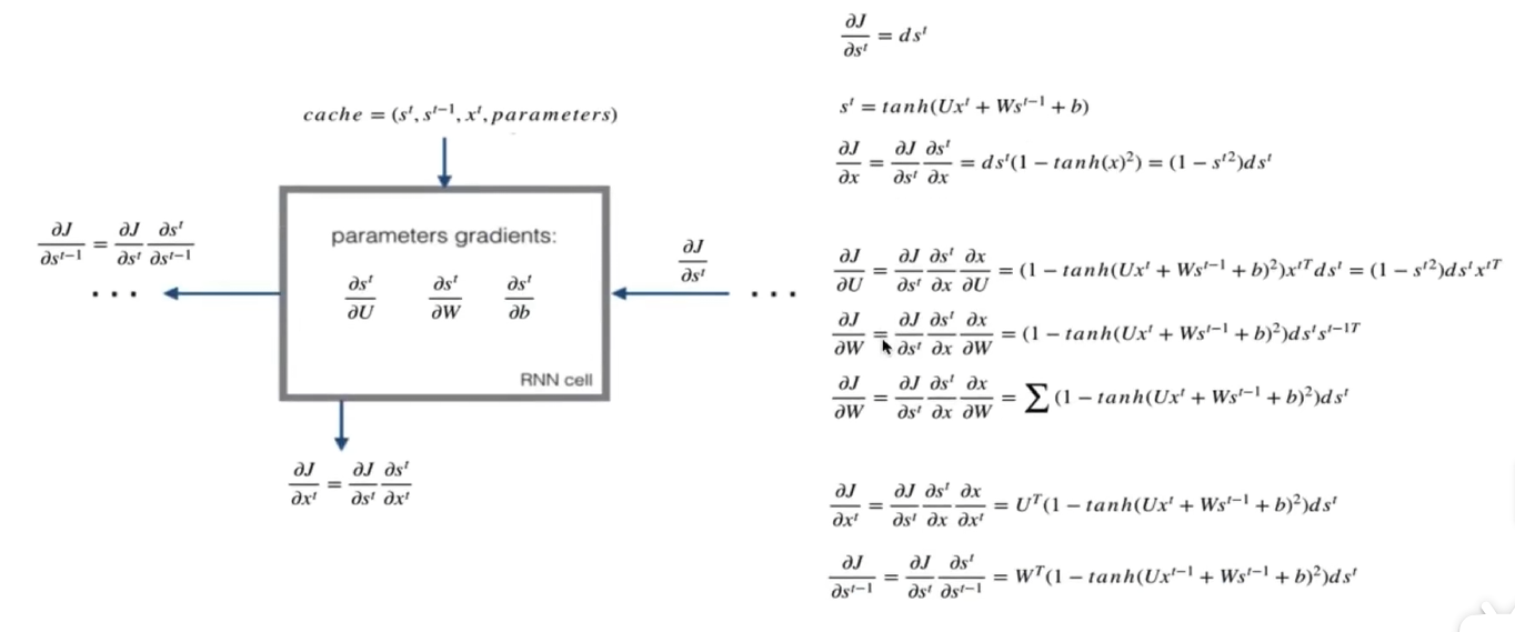
步骤
-
对于最后一个ht:计算交叉熵对于ht的梯度,记忆交叉熵对ht,V,by的梯度
∂J∂ht=dhtJ:交叉熵损失\frac{\partial J}{\partial h^t} = dh^t \\J:交叉熵损失∂ht∂J=dhtJ:交叉熵损失 -
对于前面的ht:
-
第一步:求出当前层交叉熵损失对于当前隐藏状态输出值ht的梯度+前一层相对于ht的梯度
∂J∂ht−1=∂J∂ht∂ht∂x∂x∂ht−1=dht(1−Tanh(UXt+Wht−1+bx))WT\frac{\partial J}{\partial h^{t-1}} =\frac{\partial J}{\partial h^t}\frac{\partial h^t}{\partial x}\frac{\partial x}{\partial h^{t-1}}=dh^{t}(1-Tanh(UX^t+Wh^{t-1}+b_x))W^T∂ht−1∂J=∂ht∂J∂x∂ht∂ht−1∂x=dht(1−Tanh(UXt+Wht−1+bx))WT
对于前一时刻的cell来说:
∂J∂ht=dht+dht+1(1−h(t+1)2)WT\frac{\partial J}{\partial h^t} = dh^t+dh^{t+1}(1-h^{(t+1)2})W^T∂ht∂J=dht+dht+1(1−h(t+1)2)WT
为什么是这个形式(?)- 在 RNN 的反向传播中,由于前向传播中 h^(t−1) 会影响 ht,所以损失函数 J 对 ht 的梯度会通过链式法则反向传播,影响 h^(t−1) 的梯度
-
第二步:计算tanh激活函数的梯度
∂J∂x=∂J∂ht∂ht∂x这里的x就是Tanh(x)中的xht=Tanh(x),∂ht∂x=1−Tanh(x)2=1−(ht)2∂J∂x=∂J∂ht∂ht∂x=dht(1−(ht)2)\frac{\partial J}{\partial x} = \frac{\partial J}{\partial h^t}\frac{\partial h^t}{\partial x} \\这里的x就是Tanh(x)中的x\\h^t = Tanh(x),\frac{\partial h^t}{\partial x} = 1-Tanh(x)^2=1-(h^t)^2 \\\frac{\partial J}{\partial x} = \frac{\partial J}{\partial h^t}\frac{\partial h^t}{\partial x}=dh^t(1-(h^t)^2) \\∂x∂J=∂ht∂J∂x∂ht这里的x就是Tanh(x)中的xht=Tanh(x),∂x∂ht=1−Tanh(x)2=1−(ht)2∂x∂J=∂ht∂J∂x∂ht=dht(1−(ht)2) -
计算UXt+Wht-1+bx的对于不同参数的梯度
∂J∂U=∂J∂ht∂ht∂x∂x∂U=dht(1−Tanh(UXt+Wht−1+bx)2)∂UXt∂U=dht(1−Tanh(UXt+Wht−1+bx)2)XtT=dht(1−ht2)XtT∂J∂W=∂J∂ht∂ht∂x∂x∂W=dht(1−Tanh(UXt+Wht−1+bx)2)∂Wht−1∂W=dht(1−Tanh(UXt+Wht−1+bx)2)h(t−1)T=dht(1−ht2)h(t−1)T∂J∂bx=∂J∂ht∂ht∂x∂x∂bx=∑dht(1−Tanh(UXt+Wht−1+bx)2)\frac{\partial J}{\partial U} = \frac{\partial J}{\partial h^t}\frac{\partial h^t}{\partial x}\frac{\partial x}{\partial U}=dh^t(1-Tanh(UX^t+Wh_{t-1}+b_x)^2)\frac{\partial UX^t}{\partial U}=dh^t(1-Tanh(UX^t+Wh_{t-1}+b_x)^2)X_t^T=dh^t(1-h^{t2})X^{tT}\\\frac{\partial J}{\partial W}=\frac{\partial J}{\partial h^t}\frac{\partial h^t}{\partial x}\frac{\partial x}{\partial W}=dh^t(1-Tanh(UX_t+Wh^{t-1}+b_x)^2)\frac{\partial Wh^{t-1}}{\partial W}=dh^t(1-Tanh(UX_t+Wh^{t-1}+b_x)^2)h^{(t-1)T}=dh^t(1-h^{t2})h^{(t-1)T}\\\frac{\partial J}{\partial b_x}=\frac{\partial J}{\partial h^t}\frac{\partial h^t}{\partial x}\frac{\partial x}{\partial b_x}=\sum dh^t(1-Tanh(UX_t+Wh^{t-1}+b_x)^2)\\∂U∂J=∂ht∂J∂x∂ht∂U∂x=dht(1−Tanh(UXt+Wht−1+bx)2)∂U∂UXt=dht(1−Tanh(UXt+Wht−1+bx)2)XtT=dht(1−ht2)XtT∂W∂J=∂ht∂J∂x∂ht∂W∂x=dht(1−Tanh(UXt+Wht−1+bx)2)∂W∂Wht−1=dht(1−Tanh(UXt+Wht−1+bx)2)h(t−1)T=dht(1−ht2)h(t−1)T∂bx∂J=∂ht∂J∂x∂ht∂bx∂x=∑dht(1−Tanh(UXt+Wht−1+bx)2)
为什么bx的梯度是显式求和的(?)- bx是向量而不是矩阵,U,V,W矩阵运算中已经蕴含了求和的运算
-
梯度消失和梯度爆炸
以损失函数对W的梯度为例,如果将整个式子展开:∂J∂W=∂J∂Ot∂Ot∂ht∂ht∂ht−1∂ht−1∂ht−2⋯∂h1∂W=∂J∂OtVWt−1h0出现了Wt−1这样的高次项 以损失函数对W的梯度为例,如果将整个式子展开:\\ \frac{\partial J}{\partial W}=\frac{\partial J}{\partial O^t}\frac{\partial O^t}{\partial h^t}\frac{\partial h^t}{\partial h^{t-1}}\frac{\partial h^{t-1}}{\partial h^{t-2}}\cdots\frac{\partial h^1}{\partial W}=\frac{\partial J}{\partial O^t}VW^{t-1}h^0\\ 出现了W^{t-1}这样的高次项 以损失函数对W的梯度为例,如果将整个式子展开:∂W∂J=∂Ot∂J∂ht∂Ot∂ht−1∂ht∂ht−2∂ht−1⋯∂W∂h1=∂Ot∂JVWt−1h0出现了Wt−1这样的高次项
由于矩阵的高次幂运算:
- 如果矩阵中值很小,那么相乘t-1次后,梯度将趋近于0,导致梯度消失
- 如果矩阵中值大于1,相乘t-1次后,梯度将变得非常非常大(指数增长),造成梯度爆炸
代码实现
单个cell的前向传播
ht=Tanh(UXt+Wht−1+bx)Ot=SoftMax(Vht+by) h_t = Tanh(UX_t+Wh_{t-1}+b_x)\\ O_t = SoftMax(Vh_t+b_y) ht=Tanh(UXt+Wht−1+bx)Ot=SoftMax(Vht+by)
def softMax(z):'''使用优化后解决上溢问题的softMax:param z::return:'''frac1 = np.exp(z - np.max(z))return frac1 / np.sum(frac1, axis=0)def single_cell_forward(X_t, h_prev, params):'''单个cell的前向传播:param X_t: t时刻的输入特征:param h_prev: 上一个cell隐藏状态输出:param params: 包含参数U,V,W,bx,by:return: 当前时刻隐藏状态输出h_next,输出层输出o_pred,当前单元的结果cache'''# 取出参数U = params['U']V = params['V']W = params['W']bx = params['bx']by = params['by']# 根据公式计算# 隐藏状态输出h_next = np.tanh(np.dot(U, X_t) + np.dot(W, h_prev) + bx)o_pred = softMax(np.dot(V, h_next) + by)# 保存当前单元的结果用于后续反向传播cache = (h_next, h_prev, X_t, params)return h_next, o_pred, cache
测试代码
if __name__ == '__main__':# 假设词的数量m=3,隐藏状态输出维度n=5m = 3n = 5# t时刻输入X_t = np.random.randint(1, 10, size=(m,))# 权重参数矩阵U = np.random.rand(n, m)W = np.random.rand(n, n)V = np.random.rand(m, n)# 偏置向量bx = np.random.rand(n)by = np.random.rand(m)# 参数字典params = {'U': U,'W': W,'V': V,'bx': bx,'by': by}h_next, o_pred, cache = single_cell_forward(X_t, np.zeros((n,)), params)print(f"h_next={h_next}")print(f"h_next.shape={h_next.shape}")print(f"o_pred={o_pred}")print(f"o_pred.shape={o_pred.shape}")print(f"cache = {cache}")
输出
h_next=[0.99999661 0.9999691  0.99999336 0.99999988 0.99991662]
h_next.shape=(5,)
o_pred=[0.23834357 0.50695035 0.25470609]
o_pred.shape=(3,)
cache = (array([0.99999661, 0.9999691 , 0.99999336, 0.99999988, 0.99991662]), array([0., 0., 0., 0., 0.]), array([3, 4, 5]), {'U': array([[0.33597744, 0.35199656, 0.84496558],[0.47074405, 0.69302513, 0.09902294],[0.35384033, 0.45578884, 0.67554774],[0.14627346, 0.85772316, 0.81780597],[0.40808888, 0.04529709, 0.54539319]]), 'W': array([[0.91859144, 0.84184782, 0.02552209, 0.25411668, 0.36739187],[0.40527697, 0.36003162, 0.16973184, 0.29125799, 0.33362367],[0.05788751, 0.17812644, 0.34263542, 0.04960201, 0.82176851],[0.59037533, 0.87536288, 0.69340946, 0.78051622, 0.6515424 ],[0.39472684, 0.08493311, 0.29933967, 0.29577328, 0.33738917]]), 'V': array([[0.25452628, 0.78688367, 0.14518612, 0.22140222, 0.50778923],[0.75207001, 0.83221039, 0.18424528, 0.7227862 , 0.14471663],[0.22465947, 0.29209191, 0.52763865, 0.5211864 , 0.43333206]]), 'bx': array([0.00364616, 0.85947333, 0.04511529, 0.36062377, 0.91016474]), 'by': array([0.66977852, 0.70421053, 0.65303561])})
所有cell的前向传播
要对单个cell前向传播的函数进行一点点修改
def single_cell_forward(X_t, h_prev, params):'''单个cell的前向传播:param X_t: t时刻的输入特征:param h_prev: 上一个cell隐藏状态输出:param params: 包含参数U,V,W,bx,by:return: 当前时刻隐藏状态输出h_next,输出层输出o_pred,当前单元的结果cache'''# 取出参数U = params['U']V = params['V']W = params['W']# 将向量转换为2D矩阵,因为传入X[:,:,t]时,传入的是2D矩阵(m,1),会造成维度不匹配无法广播bx = params['bx'].reshape(-1, 1)by = params['by'].reshape(-1, 1)# 根据公式计算# 隐藏状态输出h_next = np.tanh(np.dot(U, X_t) + np.dot(W, h_prev) + bx)o_pred = softMax(np.dot(V, h_next) + by)# 保存当前单元的结果用于后续反向传播cache = (h_next, h_prev, X_t, params)return h_next, o_pred, cachedef all_cell_forward(X, h_0, params):'''所有cell的前向传播:param X: T个时刻的总输入:param h_0: 初始隐藏状态输出:param params: 权重参数与偏置参数:return: 所有隐藏状态输出h,所有输出y,以及用于反向传播的cell结果cache'''# 初始化缓存caches = []# 获取输入形状 X.shape=(m,1,T):T个时刻,每个时刻输入形状都是(m,n_feature)m, _, T = X.shape# 获取隐藏状态输出的大小m, n = params['V'].shape# 初始化隐藏状态输出矩阵h以及预测输出矩阵yh = np.zeros(shape=(n, 1, T))y = np.zeros(shape=(m, 1, T))# 初始化上一层隐藏状态输出h_prev和当前层隐藏状态输出h_nexth_prev = h_0.reshape(-1, 1)h_next = None# 对时间T进行遍历for t in range(T):# 对每个时刻t的cell进行前向传播h_next, o_pred, cache = single_cell_forward(X[:, :, t], h_prev, params)# 保存t时刻的隐藏状态输出hth[:, :, t] = h_next# 保存t时刻的输出oty[:, :, t] = o_pred# 更新上一层隐藏状态输出值h_prev = h_next# 更新缓存caches.append(cache)return h, y, caches
测试代码
if __name__ == '__main__':# 假设词的数量m=3,隐藏状态输出维度n=5,总时间T=10m = 3n = 5T = 10# 所有时刻总输入X = np.random.randint(1, 10, size=(m, 1, T))X_t = np.random.randint(1, 10, size=(m,))# 权重参数矩阵U = np.random.rand(n, m)W = np.random.rand(n, n)V = np.random.rand(m, n)# 偏置向量bx = np.random.rand(n)by = np.random.rand(m)# 初始化隐藏状态输出h_0h_0 = np.zeros(shape=(n,))# 参数字典params = {'U': U,'W': W,'V': V,'bx': bx,'by': by}h, y, caches = all_cell_forward(X, h_0, params)print(f"所有隐藏状态输出:{h}")print(f"所有cell预测输出:{y}")print(f"所有cell缓存:{caches}")
输出
所有隐藏状态输出:[[[0.99989596 0.99999983 0.99999993 0.99999888 0.99999997 0.999036411.         0.99998247 0.99999142 1.        ]][[0.9999974  1.         1.         0.99999996 1.         0.999368411.         0.999999   0.99999903 1.        ]][[0.99274427 0.99997137 0.99999969 0.99999959 0.99999944 0.999517670.99999999 0.99974704 0.99998339 0.99999952]][[0.99999964 0.99999997 0.99994416 0.99999938 0.99999999 0.999999951.         0.99999956 0.99999999 0.99999568]][[0.99942773 0.99999895 0.99999973 0.99999996 0.99999998 0.999995891.         0.99999079 0.99999982 0.99999973]]]
所有cell预测输出:[[[0.21934978 0.21949408 0.21949738 0.21949465 0.21949455 0.219609950.21949456 0.2194915  0.21949495 0.21949474]][[0.47649286 0.47657329 0.47656659 0.47657372 0.47657377 0.476511970.47657378 0.47656986 0.4765736  0.47657324]][[0.30415735 0.30393263 0.30393602 0.30393162 0.30393169 0.303878090.30393167 0.30393864 0.30393145 0.30393201]]]
所有cell缓存:[(array([[0.99989596],[0.9999974 ],[0.99274427],[0.99999964],[0.99942773]]), array([[0.],[0.],[0.],[0.],[0.]]), array([[2],[6],[5]]), {'U': array([[0.61490618, 0.08635726, 0.56566348],[0.80276575, 0.01537525, 0.81718339],[0.71776414, 0.05830853, 0.12442259],[0.18527363, 0.83667306, 0.36626197],[0.6257524 , 0.34133333, 0.15498834]]), 'W': array([[0.95220483, 0.05695795, 0.20636406, 0.16052577, 0.21561851],[0.05068834, 0.14326848, 0.1643835 , 0.02233559, 0.91339931],[0.53905516, 0.00504327, 0.13940935, 0.8950894 , 0.87739331],[0.17787155, 0.49380818, 0.01113887, 0.19760187, 0.03739453],[0.91517872, 0.6822562 , 0.40819702, 0.36087719, 0.66529801]]), 'V': array([[0.01025994, 0.16599076, 0.61306243, 0.05470244, 0.74698002],[0.22759081, 0.88869816, 0.5969242 , 0.55845755, 0.05226964],[0.62164083, 0.48271867, 0.43467842, 0.03041658, 0.44611198]]), 'bx': array([0.35565501, 0.99302515, 0.40024585, 0.54560208, 0.00493241]), 'by': array([0.11708065, 0.15943099, 0.01798523])}), (array([[0.99999983],[1.        ],[0.99997137],[0.99999997],[0.99999895]]), array([[0.99989596],[0.9999974 ],[0.99274427],[0.99999964],[0.99942773]]), array([[2],[5],[8]]), {'U': array([[0.61490618, 0.08635726, 0.56566348],[0.80276575, 0.01537525, 0.81718339],[0.71776414, 0.05830853, 0.12442259],[0.18527363, 0.83667306, 0.36626197],[0.6257524 , 0.34133333, 0.15498834]]), 'W': array([[0.95220483, 0.05695795, 0.20636406, 0.16052577, 0.21561851],[0.05068834, 0.14326848, 0.1643835 , 0.02233559, 0.91339931],[0.53905516, 0.00504327, 0.13940935, 0.8950894 , 0.87739331],[0.17787155, 0.49380818, 0.01113887, 0.19760187, 0.03739453],[0.91517872, 0.6822562 , 0.40819702, 0.36087719, 0.66529801]]), 'V': array([[0.01025994, 0.16599076, 0.61306243, 0.05470244, 0.74698002],[0.22759081, 0.88869816, 0.5969242 , 0.55845755, 0.05226964],[0.62164083, 0.48271867, 0.43467842, 0.03041658, 0.44611198]]), 'bx': array([0.35565501, 0.99302515, 0.40024585, 0.54560208, 0.00493241]), 'by': array([0.11708065, 0.15943099, 0.01798523])}), (array([[0.99999993],[1.        ],[0.99999969],[0.99994416],[0.99999973]]), array([[0.99999983],[1.        ],[0.99997137],[0.99999997],[0.99999895]]), array([[6],[1],[5]]), {'U': array([[0.61490618, 0.08635726, 0.56566348],[0.80276575, 0.01537525, 0.81718339],[0.71776414, 0.05830853, 0.12442259],[0.18527363, 0.83667306, 0.36626197],[0.6257524 , 0.34133333, 0.15498834]]), 'W': array([[0.95220483, 0.05695795, 0.20636406, 0.16052577, 0.21561851],[0.05068834, 0.14326848, 0.1643835 , 0.02233559, 0.91339931],[0.53905516, 0.00504327, 0.13940935, 0.8950894 , 0.87739331],[0.17787155, 0.49380818, 0.01113887, 0.19760187, 0.03739453],[0.91517872, 0.6822562 , 0.40819702, 0.36087719, 0.66529801]]), 'V': array([[0.01025994, 0.16599076, 0.61306243, 0.05470244, 0.74698002],[0.22759081, 0.88869816, 0.5969242 , 0.55845755, 0.05226964],[0.62164083, 0.48271867, 0.43467842, 0.03041658, 0.44611198]]), 'bx': array([0.35565501, 0.99302515, 0.40024585, 0.54560208, 0.00493241]), 'by': array([0.11708065, 0.15943099, 0.01798523])}), (array([[0.99999888],[0.99999996],[0.99999959],[0.99999938],[0.99999996]]), array([[0.99999993],[1.        ],[0.99999969],[0.99994416],[0.99999973]]), array([[6],[5],[2]]), {'U': array([[0.61490618, 0.08635726, 0.56566348],[0.80276575, 0.01537525, 0.81718339],[0.71776414, 0.05830853, 0.12442259],[0.18527363, 0.83667306, 0.36626197],[0.6257524 , 0.34133333, 0.15498834]]), 'W': array([[0.95220483, 0.05695795, 0.20636406, 0.16052577, 0.21561851],[0.05068834, 0.14326848, 0.1643835 , 0.02233559, 0.91339931],[0.53905516, 0.00504327, 0.13940935, 0.8950894 , 0.87739331],[0.17787155, 0.49380818, 0.01113887, 0.19760187, 0.03739453],[0.91517872, 0.6822562 , 0.40819702, 0.36087719, 0.66529801]]), 'V': array([[0.01025994, 0.16599076, 0.61306243, 0.05470244, 0.74698002],[0.22759081, 0.88869816, 0.5969242 , 0.55845755, 0.05226964],[0.62164083, 0.48271867, 0.43467842, 0.03041658, 0.44611198]]), 'bx': array([0.35565501, 0.99302515, 0.40024585, 0.54560208, 0.00493241]), 'by': array([0.11708065, 0.15943099, 0.01798523])}), (array([[0.99999997],[1.        ],[0.99999944],[0.99999999],[0.99999998]]), array([[0.99999888],[0.99999996],[0.99999959],[0.99999938],[0.99999996]]), array([[5],[6],[6]]), {'U': array([[0.61490618, 0.08635726, 0.56566348],[0.80276575, 0.01537525, 0.81718339],[0.71776414, 0.05830853, 0.12442259],[0.18527363, 0.83667306, 0.36626197],[0.6257524 , 0.34133333, 0.15498834]]), 'W': array([[0.95220483, 0.05695795, 0.20636406, 0.16052577, 0.21561851],[0.05068834, 0.14326848, 0.1643835 , 0.02233559, 0.91339931],[0.53905516, 0.00504327, 0.13940935, 0.8950894 , 0.87739331],[0.17787155, 0.49380818, 0.01113887, 0.19760187, 0.03739453],[0.91517872, 0.6822562 , 0.40819702, 0.36087719, 0.66529801]]), 'V': array([[0.01025994, 0.16599076, 0.61306243, 0.05470244, 0.74698002],[0.22759081, 0.88869816, 0.5969242 , 0.55845755, 0.05226964],[0.62164083, 0.48271867, 0.43467842, 0.03041658, 0.44611198]]), 'bx': array([0.35565501, 0.99302515, 0.40024585, 0.54560208, 0.00493241]), 'by': array([0.11708065, 0.15943099, 0.01798523])}), (array([[0.99903641],[0.99936841],[0.99951767],[0.99999995],[0.99999589]]), array([[0.99999997],[1.        ],[0.99999944],[0.99999999],[0.99999998]]), array([[1],[8],[1]]), {'U': array([[0.61490618, 0.08635726, 0.56566348],[0.80276575, 0.01537525, 0.81718339],[0.71776414, 0.05830853, 0.12442259],[0.18527363, 0.83667306, 0.36626197],[0.6257524 , 0.34133333, 0.15498834]]), 'W': array([[0.95220483, 0.05695795, 0.20636406, 0.16052577, 0.21561851],[0.05068834, 0.14326848, 0.1643835 , 0.02233559, 0.91339931],[0.53905516, 0.00504327, 0.13940935, 0.8950894 , 0.87739331],[0.17787155, 0.49380818, 0.01113887, 0.19760187, 0.03739453],[0.91517872, 0.6822562 , 0.40819702, 0.36087719, 0.66529801]]), 'V': array([[0.01025994, 0.16599076, 0.61306243, 0.05470244, 0.74698002],[0.22759081, 0.88869816, 0.5969242 , 0.55845755, 0.05226964],[0.62164083, 0.48271867, 0.43467842, 0.03041658, 0.44611198]]), 'bx': array([0.35565501, 0.99302515, 0.40024585, 0.54560208, 0.00493241]), 'by': array([0.11708065, 0.15943099, 0.01798523])}), (array([[1.        ],[1.        ],[0.99999999],[1.        ],[1.        ]]), array([[0.99903641],[0.99936841],[0.99951767],[0.99999995],[0.99999589]]), array([[8],[7],[7]]), {'U': array([[0.61490618, 0.08635726, 0.56566348],[0.80276575, 0.01537525, 0.81718339],[0.71776414, 0.05830853, 0.12442259],[0.18527363, 0.83667306, 0.36626197],[0.6257524 , 0.34133333, 0.15498834]]), 'W': array([[0.95220483, 0.05695795, 0.20636406, 0.16052577, 0.21561851],[0.05068834, 0.14326848, 0.1643835 , 0.02233559, 0.91339931],[0.53905516, 0.00504327, 0.13940935, 0.8950894 , 0.87739331],[0.17787155, 0.49380818, 0.01113887, 0.19760187, 0.03739453],[0.91517872, 0.6822562 , 0.40819702, 0.36087719, 0.66529801]]), 'V': array([[0.01025994, 0.16599076, 0.61306243, 0.05470244, 0.74698002],[0.22759081, 0.88869816, 0.5969242 , 0.55845755, 0.05226964],[0.62164083, 0.48271867, 0.43467842, 0.03041658, 0.44611198]]), 'bx': array([0.35565501, 0.99302515, 0.40024585, 0.54560208, 0.00493241]), 'by': array([0.11708065, 0.15943099, 0.01798523])}), (array([[0.99998247],[0.999999  ],[0.99974704],[0.99999956],[0.99999079]]), array([[1.        ],[1.        ],[0.99999999],[1.        ],[1.        ]]), array([[1],[5],[5]]), {'U': array([[0.61490618, 0.08635726, 0.56566348],[0.80276575, 0.01537525, 0.81718339],[0.71776414, 0.05830853, 0.12442259],[0.18527363, 0.83667306, 0.36626197],[0.6257524 , 0.34133333, 0.15498834]]), 'W': array([[0.95220483, 0.05695795, 0.20636406, 0.16052577, 0.21561851],[0.05068834, 0.14326848, 0.1643835 , 0.02233559, 0.91339931],[0.53905516, 0.00504327, 0.13940935, 0.8950894 , 0.87739331],[0.17787155, 0.49380818, 0.01113887, 0.19760187, 0.03739453],[0.91517872, 0.6822562 , 0.40819702, 0.36087719, 0.66529801]]), 'V': array([[0.01025994, 0.16599076, 0.61306243, 0.05470244, 0.74698002],[0.22759081, 0.88869816, 0.5969242 , 0.55845755, 0.05226964],[0.62164083, 0.48271867, 0.43467842, 0.03041658, 0.44611198]]), 'bx': array([0.35565501, 0.99302515, 0.40024585, 0.54560208, 0.00493241]), 'by': array([0.11708065, 0.15943099, 0.01798523])}), (array([[0.99999142],[0.99999903],[0.99998339],[0.99999999],[0.99999982]]), array([[0.99998247],[0.999999  ],[0.99974704],[0.99999956],[0.99999079]]), array([[3],[8],[3]]), {'U': array([[0.61490618, 0.08635726, 0.56566348],[0.80276575, 0.01537525, 0.81718339],[0.71776414, 0.05830853, 0.12442259],[0.18527363, 0.83667306, 0.36626197],[0.6257524 , 0.34133333, 0.15498834]]), 'W': array([[0.95220483, 0.05695795, 0.20636406, 0.16052577, 0.21561851],[0.05068834, 0.14326848, 0.1643835 , 0.02233559, 0.91339931],[0.53905516, 0.00504327, 0.13940935, 0.8950894 , 0.87739331],[0.17787155, 0.49380818, 0.01113887, 0.19760187, 0.03739453],[0.91517872, 0.6822562 , 0.40819702, 0.36087719, 0.66529801]]), 'V': array([[0.01025994, 0.16599076, 0.61306243, 0.05470244, 0.74698002],[0.22759081, 0.88869816, 0.5969242 , 0.55845755, 0.05226964],[0.62164083, 0.48271867, 0.43467842, 0.03041658, 0.44611198]]), 'bx': array([0.35565501, 0.99302515, 0.40024585, 0.54560208, 0.00493241]), 'by': array([0.11708065, 0.15943099, 0.01798523])}), (array([[1.        ],[1.        ],[0.99999952],[0.99999568],[0.99999973]]), array([[0.99999142],[0.99999903],[0.99998339],[0.99999999],[0.99999982]]), array([[5],[1],[9]]), {'U': array([[0.61490618, 0.08635726, 0.56566348],[0.80276575, 0.01537525, 0.81718339],[0.71776414, 0.05830853, 0.12442259],[0.18527363, 0.83667306, 0.36626197],[0.6257524 , 0.34133333, 0.15498834]]), 'W': array([[0.95220483, 0.05695795, 0.20636406, 0.16052577, 0.21561851],[0.05068834, 0.14326848, 0.1643835 , 0.02233559, 0.91339931],[0.53905516, 0.00504327, 0.13940935, 0.8950894 , 0.87739331],[0.17787155, 0.49380818, 0.01113887, 0.19760187, 0.03739453],[0.91517872, 0.6822562 , 0.40819702, 0.36087719, 0.66529801]]), 'V': array([[0.01025994, 0.16599076, 0.61306243, 0.05470244, 0.74698002],[0.22759081, 0.88869816, 0.5969242 , 0.55845755, 0.05226964],[0.62164083, 0.48271867, 0.43467842, 0.03041658, 0.44611198]]), 'bx': array([0.35565501, 0.99302515, 0.40024585, 0.54560208, 0.00493241]), 'by': array([0.11708065, 0.15943099, 0.01798523])})]
单个cell的反向传播
由图中确定的需要计算的梯度变量
- dh_next:当前cell的损失对输出h^t的导数
- dtanh:当前cell的损失对激活函数tanh(x)的导数
- dx_t:当前cell的损失对输入x_t的导数
- dU:表示当前cell的损失对U的导数
- dh_prev:当前cell的损失对上一个cell的隐藏状态输出的梯度
- dW:当前cell的损失对W的导数
- dbx:当前cell的损失对bx的导数
def single_cell_bp(dh_next, cache):"""单个cell的反向传播:param dh_next: 当前隐藏状态输出相对于损失函数的梯度:param cache: 当前cell的缓存:return: 梯度字典gradient"""(h_next, h_prev, X_t, params) = cache# 取出参数U = params['U']W = params['W']# 计算cell损失函数对激活函数的梯度# *:逐元素相乘而不是矩阵乘法dtanh = (1 - h_next ** 2) * dh_next# 计算cell的损失对U的梯度dU = np.dot(dtanh, X_t.T)# 计算cell的损失对W的梯度dW = np.dot(dtanh, h_prev.T)# 计算cell的损失对bx的梯度,保持维度不变dbx = np.sum(dtanh, axis=1, keepdims=1)# print(f"dbx.shape={dbx.shape}")# 计算Xt的梯度dx_t = np.dot(U.T, dtanh)# 计算h_t-1的梯度dh_prev = np.dot(W.T, dtanh)# 所有的梯度保存到字典中gradient = {"dtanh": dtanh,"dU": dU,"dW": dW,"dbx": dbx,"dx_t": dx_t,"dh_prev": dh_prev}return gradient
所有cell的反向传播
- 最后一个cell和其他cell,ht的梯度的组成不一样
- 不同时刻对于参数U,V,W,b的梯度需要相加
def rnn_backpagation(dh, caches):"""所有cell的反向传播:param dh: 每个时刻的损失对其当前隐藏状态输出的梯度(假设已知),shape=(n,1,T):param caches: 所有cell的缓存:return: 梯度字典向量gradients"""# 获取总时刻T以及隐藏状态输出大小nn, _, T = dh.shape# 获取t时刻输入的长度(h1, h0, X1, params) = caches[0]m, _ = X1.shape# 初始化# 参数梯度dU = np.zeros(shape=(n, m))dW = np.zeros(shape=(n, n))dbx = np.zeros(shape=(n, 1))# 第二部分梯度值dh_prevt = np.zeros(shape=(n, 1))# 不需要更新的梯度:所有x_t的梯度dxdx = np.zeros(shape=(m, 1, T))# 循环从后往前计算梯度for t in reversed(range(T)):# 从最后一个时刻T开始,T-1->1时刻ht梯度由两部分组成gradient = single_cell_bp(dh[:, :, t] + dh_prevt, caches[t])# 更新第二部分ht梯度dh_prevt = gradient['dh_prev']# 当前时刻共享参数的梯度dUt = gradient['dU']dWt = gradient['dW']dbxt = gradient['dbx']# x_t的梯度值dx_t = gradient['dx_t']# 共享参数的梯度累加dU += dUtdW += dWtdbx += dbxt# 每个时刻对输入x的梯度dx[:, :, t] = dx_tgradients = {"dU": dU,"dW": dW,"dbx": dbx,"dx": dx,}return gradients
测试代码
if __name__ == '__main__':# 假设词的数量m=3,隐藏状态输出维度n=5,总时间T=10m = 3n = 5T = 10# 所有时刻总输入X = np.random.randint(1, 10, size=(m, 1, T))# 权重参数矩阵U = np.random.rand(n, m)W = np.random.rand(n, n)V = np.random.rand(m, n)# 偏置向量bx = np.random.rand(n)by = np.random.rand(m)# 初始化隐藏状态输出h_0h_0 = np.zeros(shape=(n,))# 参数字典params = {'U': U,'W': W,'V': V,'bx': bx,'by': by}# 前向传播获取每个cell的缓存cachesh, y, caches = all_cell_forward(X, h_0, params)# 每个时刻的损失对其当前隐藏状态输出的梯度dh = np.random.rand(n, 1, T)gradients = rnn_backpagation(dh, caches)print(gradients)
输出结果
{'dU': array([[6.49540232e-06, 3.72579122e-06, 3.23351186e-06],[4.37638801e-03, 2.40148936e-03, 2.23775248e-03],[3.23720391e-05, 1.61878844e-05, 1.61879888e-05],[1.20912365e-07, 6.09633400e-08, 6.04361416e-08],[8.37521326e-05, 2.06390984e-04, 3.08098966e-05]]), 'dW': array([[3.14708439e-06, 3.14695660e-06, 3.14708440e-06, 3.14708441e-06,3.14708344e-06],[2.11033175e-03, 2.11024002e-03, 2.11033175e-03, 2.11033177e-03,2.11032984e-03],[1.61852431e-05, 1.61845877e-05, 1.61852431e-05, 1.61852431e-05,1.61852391e-05],[6.03264487e-08, 6.03240020e-08, 6.03264489e-08, 6.03264490e-08,6.03264323e-08],[8.92882278e-06, 8.92842339e-06, 8.92882273e-06, 8.92882292e-06,8.92881746e-06]]), 'dbx': array([[3.20862272e-06],[2.12037255e-03],[1.61853782e-05],[6.03727971e-08],[3.08095836e-05]]), 'dx': array([[[1.28698441e-05, 6.50495348e-06, 2.98409670e-04, 2.41618289e-07,2.37413386e-09, 1.48155122e-08, 2.45888172e-06, 1.21666503e-09,6.32489046e-09, 1.66698702e-07]],[[9.45749729e-06, 1.94154493e-05, 8.66429866e-04, 7.05815250e-07,7.13539950e-09, 4.45427660e-08, 7.38876306e-06, 3.65828721e-09,1.90159891e-08, 5.01228253e-07]],[[2.47229069e-05, 1.54962205e-05, 6.96851125e-04, 5.72608705e-07,5.66545602e-09, 3.53662058e-08, 5.86642385e-06, 2.90464334e-09,1.50992307e-08, 3.97969919e-07]]])}
GRU(门控循环单元)
什么是GRU
仍然是两个输入:
- t时刻特征xt
- 上一时刻隐藏状态输出h_t-1
2个输出:
- 当前时刻隐藏状态输出ht
- 输出层预测输出Ot
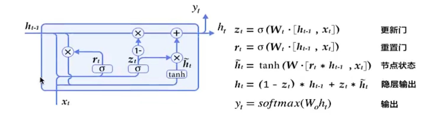
但是内部结构发生了变化,新增了两个门,重置门(Reset gate)与更新门(Update gate)
-
重置门决定了如何将新的输入信息与前面的记忆相结合
rt=σ(Wt⋅[ht−1,xt])σ:sigmoid(x)r_t =\sigma(W_t\cdot[h_{t-1},x_t])\\\sigma:sigmoid(x)rt=σ(Wt⋅[ht−1,xt])σ:sigmoid(x) -
更新门定义了前面记忆保存到当前时间步的量
zt=σ(Wt⋅[ht−1,xt])z_t = \sigma(W_t\cdot[h_{t-1},x_t])zt=σ(Wt⋅[ht−1,xt]) -
节点状态
ht~=Tanh(W⋅[rt∗ht−1,xt])将重置门设为1,更新门设为0:ht~=Tanh(W⋅[ht−1,xt])等于标准RNN的ht\tilde{h_t} = Tanh(W\cdot[r_t*h_{t-1},x_t])\\将重置门设为1,更新门设为0:\\\tilde{h_t}= Tanh(W\cdot[h_{t-1},x_t])\\等于标准RNN的h_tht~=Tanh(W⋅[rt∗ht−1,xt])将重置门设为1,更新门设为0:ht~=Tanh(W⋅[ht−1,xt])等于标准RNN的ht -
隐藏状态输出
ht=(1−zt)∗ht−1+zt∗ht~h_t = (1-z_t)*h_{t-1}+z_t*\tilde{h_t}ht=(1−zt)∗ht−1+zt∗ht~ -
输出
yt=softMax(Woht)y_t = softMax(W_oh_t)yt=softMax(Woht)
直观理解

GRU会记住cat这个位置是1,直到was的位置,选择was而不是were
本质解决问题
-
为了解决短期记忆问题,每个能够自适应捕捉不同尺度的依赖关系
-
解决梯度消失的问题,在隐层输出的地方ht,ht-1的关系用加法而不是RNN中乘法+激活函数
使用:ht=(1−zt)∗ht−1+zt∗ht~而不是ht=tanh(W⋅[ht−1,Xt])避免了出现梯度消失和梯度爆炸使用:h_t = (1-z_t)*h_{t-1}+z_t*\tilde{h_t}\\而不是h_t = tanh(W\cdot[h_{t-1},X_t]) \\避免了出现梯度消失和梯度爆炸使用:ht=(1−zt)∗ht−1+zt∗ht~而不是ht=tanh(W⋅[ht−1,Xt])避免了出现梯度消失和梯度爆炸
LSTM(长短记忆网络)
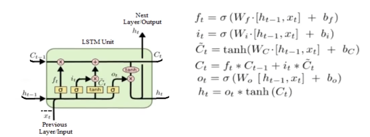
ft=σ(Ufxt+Wfht−1+bf)(遗忘门)it=σ(Uixt+Wiht−1+bi)(输入门)c~t=tanh(Ucxt+Wcht−1+bc)ct=ft∗ct−1+it∗c~tot=σ(Uoxt+Woht−1+bo)(输出门)ht=ot∗tanh(ct)
f^t = \sigma(U^fx^t+W^fh^{t-1}+b^f)(遗忘门)\\
i^t =\sigma(U^ix^t+W^ih^{t-1}+b^i)(输入门)\\
\tilde{c}^t = tanh(U^cx^t+W^ch^{t-1}+b^c)\\
c^t = f^t*c^{t-1}+i^t*\tilde{c}^t\\
o^t = \sigma(U^ox^t+W^oh^{t-1}+b^o)(输出门)\\
h^t = o^t*tanh(c^t)\\
\\
ft=σ(Ufxt+Wfht−1+bf)(遗忘门)it=σ(Uixt+Wiht−1+bi)(输入门)c~t=tanh(Ucxt+Wcht−1+bc)ct=ft∗ct−1+it∗c~tot=σ(Uoxt+Woht−1+bo)(输出门)ht=ot∗tanh(ct)
- ht为该cell单元的输出
- ct为隐藏状态
- 三个门:遗忘门f,输入门i,输出门o
- 遗忘门(forget gate):决定有多少旧信息被保留。
- 输入门/更新门(input gate):决定有多少新信息被写入记忆单元。
- 输出门(output gate):决定有多少记忆单元的信息被输出
作用
便于记忆更长距离的时间状态
RNN案例
前置知识
set(text):将文本转换为一个集合,去除重复字符
eg:
str = "aaaa"
str = set(str)
print(str)
# {'a'}
list():转换为列表
str = "aaaa"
str = list(set(str))
print(str)
# ['a']
enumerate(text):参数转换为字典,索引+元素的形式
str = "Hello"for i, c in enumerate(str):print(f"i={i},c={c}")
i=0,c=H
i=1,c=e
i=2,c=l
i=3,c=l
i=4,c=o
np.eye():将普通向量进行one-hot编码
x = np.array([1, 2, 3, 4])one_hot = np.eye(x.shape[0] + 1)[x]
print(one_hot)
[[0. 1. 0. 0. 0.][0. 0. 1. 0. 0.][0. 0. 0. 1. 0.][0. 0. 0. 0. 1.]]
用法:可以构建字符的唯一整数索引,同时也可以构造整数索引映射回原始字符
text = "Heello World"
# set()去重后用list()转换为列表进行排序
chars = sorted(list(set(text)))# 字符的唯一整数索引 K:V = char:int
char_to_idx = {c: i for i, c in enumerate(chars)}
# 通过索引找到对应字符 K:V = int:char
idx_to_char = {i: c for i, c in enumerate(chars)}
char_to_idx={' ': 0, 'H': 1, 'W': 2, 'd': 3, 'e': 4, 'l': 5, 'o': 6, 'r': 7}
idx_to_char={0: ' ', 1: 'H', 2: 'W', 3: 'd', 4: 'e', 5: 'l', 6: 'o', 7: 'r'}
torch.tensor.unsqueeze():指定张量增加的维度
import torchlist = [[1, 2], [3, 4], [5, 6]]
list_tensor = torch.tensor(list, dtype=torch.float32)
print(f"list_tensor.shape={list_tensor.shape}")list_tensor = list_tensor.unsqueeze(0)
print(f"unsqueeze(0):list_tensor.shape={list_tensor.shape}")
list_tensor.shape=torch.Size([3, 2])
unsqueeze(0):list_tensor.shape=torch.Size([1, 3, 2])
torch.tensor.squeeze():去掉张量中长度为1的维度
import torchlist = [[1, 2], [3, 4], [5, 6]]
list_tensor = torch.tensor(list, dtype=torch.float32)
print(f"list_tensor.shape={list_tensor.shape}")list_tensor = list_tensor.unsqueeze(0)
print(f"unsqueeze(0):list_tensor.shape={list_tensor.shape}")
list_tensor = list_tensor.squeeze()
print(f"squeeze():list_tensor.shape={list_tensor.shape}")
list_tensor.shape=torch.Size([3, 2])
unsqueeze(0):list_tensor.shape=torch.Size([1, 3, 2])
squeeze():list_tensor.shape=torch.Size([3, 2])
预测文本输入
依赖
from shlex import joinimport torch
import torch.nn as nn
import torch.optim as optim
import numpy as np
文本初步处理
# 文本
text = ":Hello World!"# 构造词典
chars = sorted(list(set(text)))
char_to_idx = {c: i for i, c in enumerate(chars)}
print(f"char_to_idx = {char_to_idx}")
idx_to_char = {i: c for i, c in enumerate(chars)}
print(f"idx_to_char = {idx_to_char}")
char_to_idx = {' ': 0, '!': 1, ':': 2, 'H': 3, 'W': 4, 'd': 5, 'e': 6, 'l': 7, 'o': 8, 'r': 9}
idx_to_char = {0: ' ', 1: '!', 2: ':', 3: 'H', 4: 'W', 5: 'd', 6: 'e', 7: 'l', 8: 'o', 9: 'r'}
处理输入数据与真实目标
# 输入与目标
input_str = ":Hello World!"
target_str = "Hello World!:"# 转换为索引
input_data = [char_to_idx[c] for c in input_str]
target_data = [char_to_idx[c] for c in target_str]# 对输入进行 one-hot 编码
# shape=(len(input_data),len(char_to_idx))
X = np.eye(len(char_to_idx))[input_data]# 转为张量
# 在第0维添加维度 [1, seq_len, input_size],nn.RNN输入形状为[batch_size,seq_len,input_size]
X = torch.tensor(X, dtype=torch.float32).unsqueeze(0)
# print(f"X.shape={X.shape}")
y = torch.tensor(target_data, dtype=torch.long)
RNN模型
class RNN(nn.Module):def __init__(self, input_size, hidden_size, output_size):# 调用父类对rnn等属性初始化super(RNN, self).__init__()# 输入格式为[batch_size,seq_len,input_size](因为指定了batch_first=True)self.rnn = nn.RNN(input_size, hidden_size, batch_first=True)# 全连接层self.fc = nn.Linear(hidden_size, output_size)# 前向传播def forward(self, x, hidden=None):# cell输出以及隐藏状态输出out, hidden = self.rnn(x, hidden)# 全连接层输出logits = self.fc(out)return logits, hidden
训练模型
# 参数
input_size = len(char_to_idx)
hidden_size = 128
output_size = len(char_to_idx)
epochs = 100# 实例化模型
model = RNN(input_size, hidden_size, output_size)# 损失函数和优化器
criterion = nn.CrossEntropyLoss()
optimizer = optim.Adam(model.parameters(), lr=0.01)# 初始化隐藏状态
hidden = torch.zeros(1, 1, hidden_size)  # [num_layers, batch_size, hidden_size]# 训练循环
for epoch in range(epochs):# 将模型设置为训练模式model.train()# 清空优化器中所有参数的梯度缓存optimizer.zero_grad()# 前向传播# 使用detach切断历史梯度logits, hidden = model(X, hidden.detach())# 计算损失loss = criterion(logits.view(-1, output_size), y)# 反向传播和优化loss.backward()optimizer.step()if (epoch + 1) % 10 == 0:print(f"Epoch [{epoch + 1}/{epochs}], Loss: {loss.item():.4f}")
验证代码
hidden = None
# logits.shape=[batch_size,seq_len,input_size]
logits, _ = model(X, hidden)# 找到在input_size上最大值索引,即最可能出现的字符
# 使用squeeze将长度为1的维度去掉,[1,seq_len] -> [seq_len]
# 转换为numpy形式向量
pred = torch.argmax(logits, dim=2).squeeze().numpy()
# print(f"pred={pred}")
# print(f"pred={pred.shape}")pred_res = join([idx_to_char[i] for i in pred])
print(pred_res)
预测结果
Epoch [100/100], Loss: 0.0041
RNN预测输出:H e l l o ' ' W o r l d '!' :