【机器学习实战】七、梯度下降
梯度下降
一、线性回归
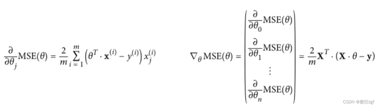
线性回归算法推导过程可以基于最小二乘法直接求解,但这并不是机器学习的思想,由此引入了梯度下降方法。本文讲解其中每一步流程与实验对比分析。
1.初始化
import numpy as np
import os
%matplotlib inline
import matplotlib
import matplotlib.pyplot as plt
plt.rcParams['axes.labelsize'] = 14
plt.rcParams['xtick.labelsize'] = 12
plt.rcParams['ytick.labelsize'] = 12
import warnings
warnings.filterwarnings('ignore')
np.random.seed(42)
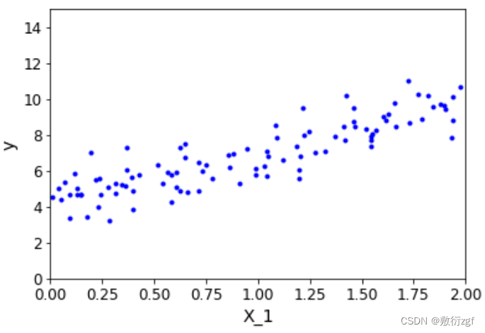
2.回归方程

import numpy as np
X = 2*np.random.rand(100,1)
y = 4+ 3*X +np.random.randn(100,1)
plt.plot(X,y,'b.')
plt.xlabel('X_1')
plt.ylabel('y')
plt.axis([0,2,0,15])
plt.show()
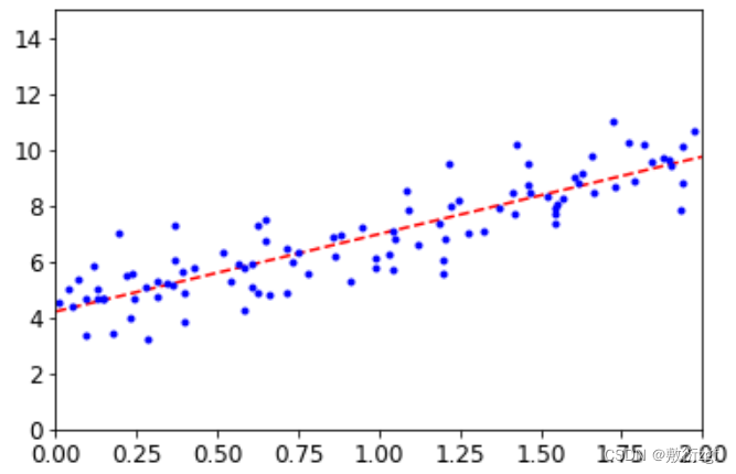
X_b = np.c_[np.ones((100,1)),X]
theta_best = np.linalg.inv(X_b.T.dot(X_b)).dot(X_b.T).dot(y)
print(theta_best)
# 输出 :
array([[4.21509616],[2.77011339]])
X_new = np.array([[0],[2]])
X_new_b = np.c_[np.ones((2,1)),X_new]
y_predict = X_new_b.dot(theta_best)
print(y_predict)
# 输出:
array([[4.21509616],[9.75532293]])
plt.plot(X_new,y_predict,'r--')
plt.plot(X,y,'b.')
plt.axis([0,2,0,15])
plt.show()
二、调用sklearn API
sklearnAPI官网: https://scikit-learn.org/stable/modules/classes.html
from sklearn.linear_model import LinearRegression
lin_reg = LinearRegression()
lin_reg.fit(X,y)
print (lin_reg.coef_)
print (lin_reg.intercept_)
#
[[2.77011339]]
[4.21509616]
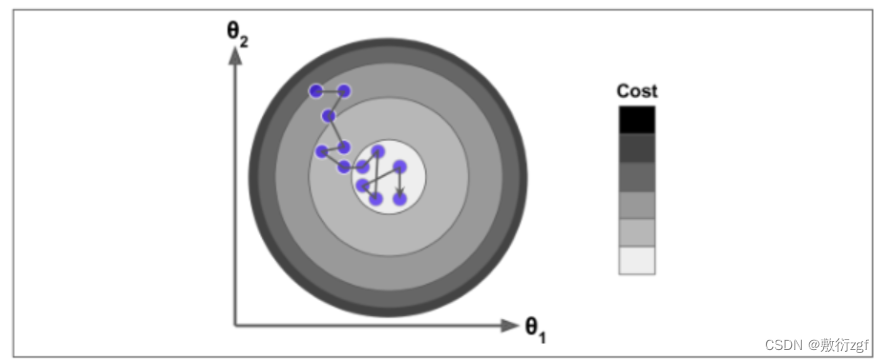
三、梯度下降
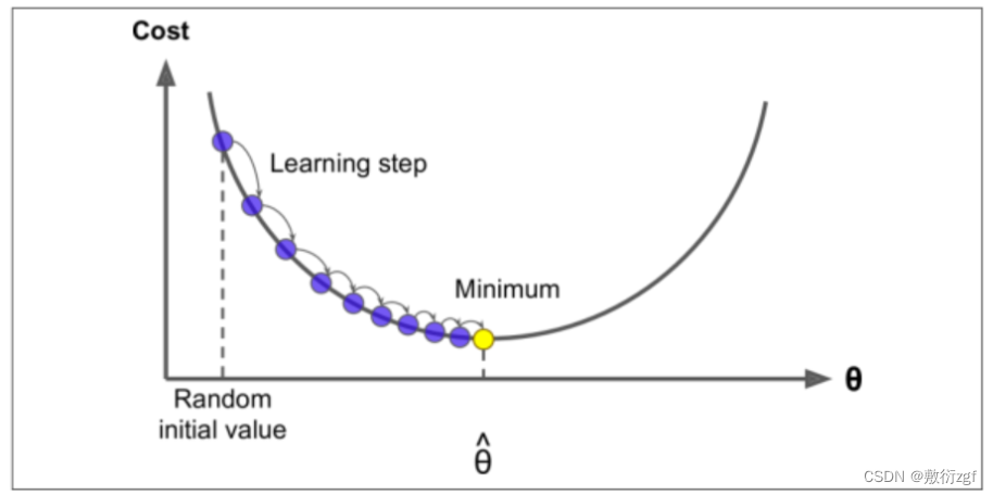
当步长较小时,训练次数较多;
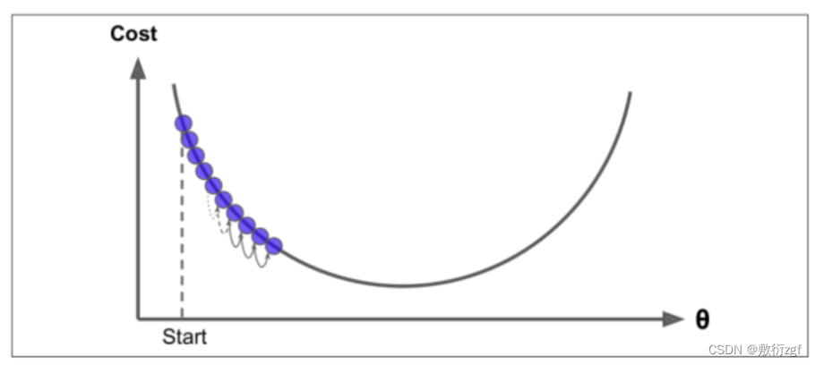
当步长较大时,波动大;
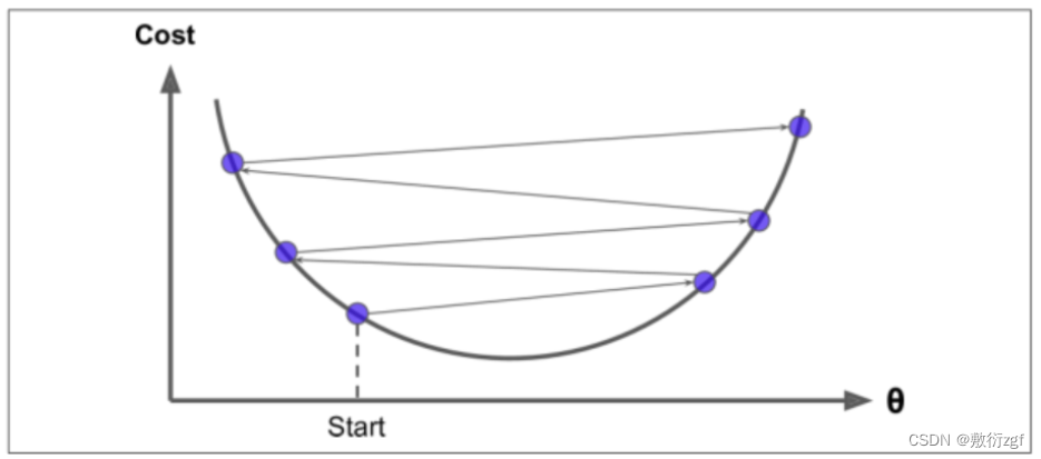
学习率应当尽可能小,随着迭代的进行应当越来越小。
1.批量梯度下降
eta = 0.1 #学习率
n_iterations = 1000 # 迭代次数
m = 100
theta = np.random.randn(2,1) # 随机初始化参数theta
for iteration in range(n_iterations):gradients = 2/m* X_b.T.dot(X_b.dot(theta)-y)theta = theta - eta*gradients
theta
#
array([[4.21509616],[2.77011339]])
X_new_b.dot(theta)
#
array([[4.21509616],[9.75532293]])
theta_path_bgd = []
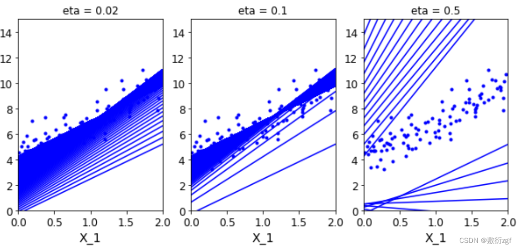
def plot_gradient_descent(theta,eta,theta_path = None):m = len(X_b)plt.plot(X,y,'b.')n_iterations = 1000for iteration in range(n_iterations):y_predict = X_new_b.dot(theta)plt.plot(X_new,y_predict,'b-')gradients = 2/m* X_b.T.dot(X_b.dot(theta)-y)theta = theta - eta*gradientsif theta_path is not None:theta_path.append(theta)plt.xlabel('X_1')plt.axis([0,2,0,15])plt.title('eta = {}'.format(eta))
theta = np.random.randn(2,1)plt.figure(figsize=(10,4))
plt.subplot(131)
plot_gradient_descent(theta,eta = 0.02)
plt.subplot(132)
plot_gradient_descent(theta,eta = 0.1,theta_path=theta_path_bgd)
plt.subplot(133)
plot_gradient_descent(theta,eta = 0.5)
plt.show()
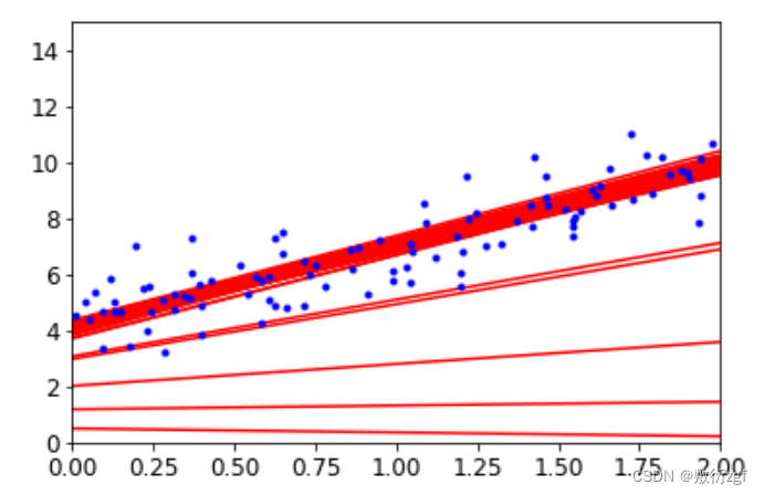
2.随机梯度下降
theta_path_sgd=[]
m = len(X_b)
np.random.seed(42)
n_epochs = 50
t0 = 5
t1 = 50def learning_schedule(t):return t0/(t1+t)
theta = np.random.randn(2,1)for epoch in range(n_epochs):for i in range(m):if epoch < 10 and i<10:y_predict = X_new_b.dot(theta)plt.plot(X_new,y_predict,'r-')random_index = np.random.randint(m)xi = X_b[random_index:random_index+1]yi = y[random_index:random_index+1]gradients = 2* xi.T.dot(xi.dot(theta)-yi)eta = learning_schedule(epoch*m+i)theta = theta-eta*gradientstheta_path_sgd.append(theta)plt.plot(X,y,'b.')
plt.axis([0,2,0,15])
plt.show()
3.MiniBatch梯度下降
theta_path_mgd=[]
n_epochs = 50
minibatch = 16
theta = np.random.randn(2,1)
t0, t1 = 200, 1000
def learning_schedule(t):return t0 / (t + t1)
np.random.seed(42)
t = 0
for epoch in range(n_epochs):shuffled_indices = np.random.permutation(m)X_b_shuffled = X_b[shuffled_indices]y_shuffled = y[shuffled_indices]for i in range(0,m,minibatch):t+=1xi = X_b_shuffled[i:i+minibatch]yi = y_shuffled[i:i+minibatch]gradients = 2/minibatch* xi.T.dot(xi.dot(theta)-yi)eta = learning_schedule(t)theta = theta-eta*gradientstheta_path_mgd.append(theta)
theta
#
array([[4.25490684],[2.80388785]])
四、3种策略的对比实验
theta_path_bgd = np.array(theta_path_bgd)
theta_path_sgd = np.array(theta_path_sgd)
theta_path_mgd = np.array(theta_path_mgd)
plt.figure(figsize=(12,6))
plt.plot(theta_path_sgd[:,0],theta_path_sgd[:,1],'r-s',linewidth=1,label='SGD')
plt.plot(theta_path_mgd[:,0],theta_path_mgd[:,1],'g-+',linewidth=2,label='MINIGD')
plt.plot(theta_path_bgd[:,0],theta_path_bgd[:,1],'b-o',linewidth=3,label='BGD')
plt.legend(loc='upper left')
plt.axis([3.5,4.5,2.0,4.0])
plt.show()
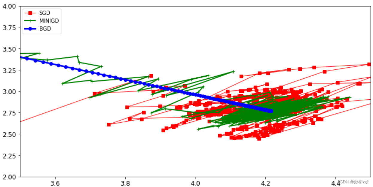
实际当中用minibatch比较多,一般情况下选择batch数量应当越大越好。