[Computer Vision]实验三:图像拼接
目录
一、实验内容
二、实验过程及结果
2.1 单应性变换
2.2 RANSAC算法
三、实验小结
一、实验内容
- 理解单应性变换中各种变换的原理(自由度),并实现图像平移、旋转、仿射变换等操作,输出对应的单应性矩阵。
- 利用RANSAC算法优化关键点匹配,比较优化前后图像拼接和所生成全景图的差别,输出RANSAC前后匹配点数量、单应性矩阵。
二、实验过程及结果
2.1 单应性变换
(1)实验代码
import cv2
from networkx import center
import numpy as np
from scipy.fft import dst
import matplotlib.pyplot as plt
img=cv2.imread("D:/Computer vision/test1 picture/picture3.png")x=100
y=50
M0=np.float32([[1,0,x],[0,1,y]])
translated=cv2.warpAffine(img,M0,(img.shape[1],img.shape[0]))
print("平移变换单应性矩阵:\n",M0)img_center=(img.shape[1]/2,img.shape[0]/2)
M1=cv2.getRotationMatrix2D(img_center,45,1)
rotated=cv2.warpAffine(img,M1,(img.shape[1],img.shape[0]))
print("旋转变换单应性矩阵:\n",M1)M2=cv2.getRotationMatrix2D(img_center,0,0.5)
scaled=cv2.warpAffine(img,M2,(img.shape[1],img.shape[0]))
print("缩放变换单应性矩阵:\n",M2)rows,cols,ch=img.shape
src_points=np.float32([[0,0],[cols-1,0],[0,rows-1]])
dst_points=np.float32([[0,rows*0.33],[cols*0.85,rows*0.25],[cols*0.15,rows*0.7]])
M3=cv2.getAffineTransform(src_points,dst_points)
warped=cv2.warpAffine(img,M3,(cols,rows))
print("扭曲变换单应性矩阵:\n",M3)rows,cols=img.shape[:2]
pts1=np.float32([[150,50],[400,50],[60,450],[310,450]])
pts2=np.float32([[50,50],[rows-50,50],[50,cols-50],[rows-50,cols-50]])
M4=cv2.getPerspectiveTransform(pts1,pts2)
img_dst=cv2.warpPerspective(img,M4,(cols,rows))
print("透视变换单应性矩阵:\n",M4)plt.figure("Processed Images")
plt.subplot(2,3,1)
plt.imshow(img)
plt.title("Original Image")
plt.subplot(2,3,2)
plt.imshow(translated)
plt.title("Translated Image")
plt.subplot(2,3,3)
plt.imshow(rotated)
plt.title("Rotated Image")
plt.subplot(2,3,4)
plt.imshow(scaled)
plt.title("Scaled Image")
plt.subplot(2,3,5)
plt.imshow(warped)
plt.title("Warped Image")
plt.subplot(2,3,6)
plt.imshow(img_dst)
plt.title("Dst Image")
plt.show()
plt.savefig("D:/Computer vision/ransac_picture/processed_images.png")
plt.show()
(2)实验结果截图
图1为输出的单应性矩阵结果截图:
平移变换:两个自由度(两个平移参数),单应性矩阵为2*3的矩阵
旋转变换:一个自由度(一个旋转角度参数),单应性矩阵为2*3的矩阵
缩放变换:一个自由度(一个缩放因子),单应性矩阵为2*3的矩阵
扭曲变换有六个自由度(两个旋转参数 一个缩放因子),单应性矩阵为2*3的矩阵
透视变换有八个自由度(5个是仿射变换参数,3个是透视变换参数),单应性矩阵为3*3的矩阵
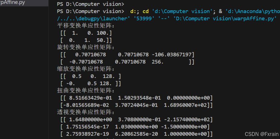
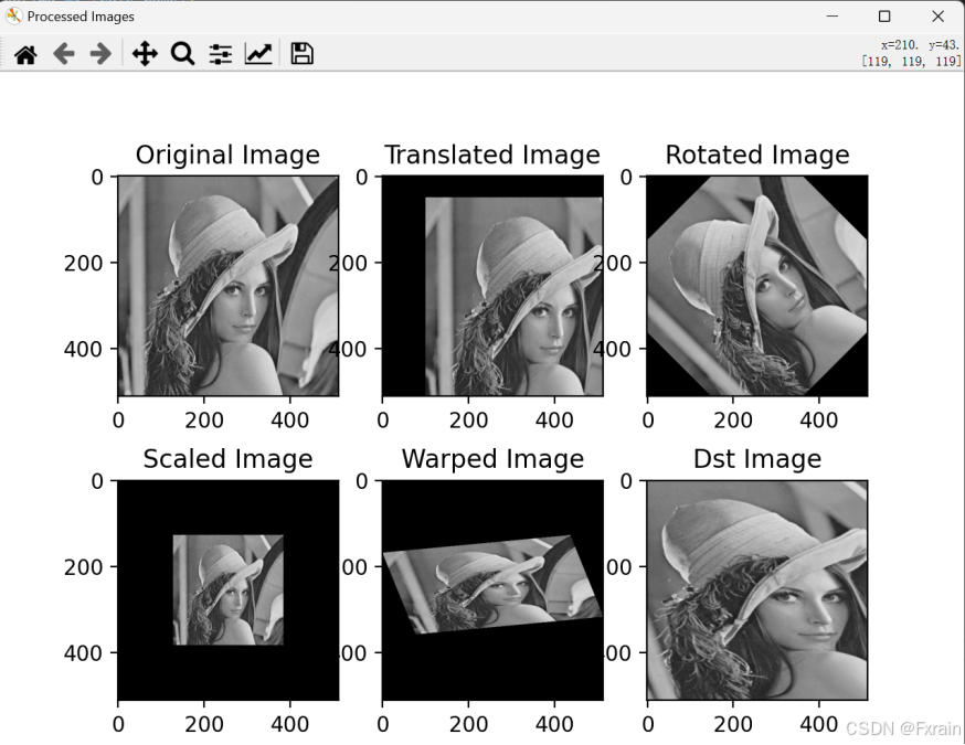
图2为输出的单应性变换的结果图:
可以看到,平移变换的图像在x方向上平移100个像素,在y方向上平移50个像素。旋转变换的图像绕图像中心旋转45度。缩放变换的图像在x方向上缩小到原来的一半,在y方向上缩小到原来的一半。扭曲变换的图像进行仿射变换,包括旋转、缩放、平移和剪切。透视变换的图像进行了透视变换,包括旋转、缩放、平移和透视变形。
2.2 RANSAC算法
(1)实验代码
import cv2
import numpy as npdef detectAndCompute(image):gray = cv2.cvtColor(image, cv2.COLOR_BGR2GRAY)sift = cv2.SIFT_create()keypoints, descriptors = sift.detectAndCompute(gray, None)return keypoints, descriptorsdef matchKeyPoints(kpsA, kpsB, featuresA, featuresB, ratio=0.75, reprojThresh=4.0):matcher = cv2.BFMatcher()rawMatches = matcher.knnMatch(featuresA, featuresB, 2)matches = []for m in rawMatches:if len(m) == 2 and m[0].distance < ratio * m[1].distance:matches.append((m[0].queryIdx, m[0].trainIdx))ptsA = np.float32([kpsA[i].pt for (i, _) in matches])ptsB = np.float32([kpsB[i].pt for (_, i) in matches])(M, status) = cv2.findHomography(ptsA, ptsB, cv2.RANSAC, reprojThresh)return (M, matches, status)def drawMatches(imgA, imgB, kpsA, kpsB, matches, status):(hA, wA) = imgA.shape[:2](hB, wB) = imgB.shape[:2]result = np.zeros((max(hA, hB), wA + wB, 3), dtype="uint8")result[0:hA, 0:wA] = imgAresult[0:hB, wA:] = imgBfor ((trainIdx, queryIdx), s) in zip(matches, status):if s == 1:ptA = (int(kpsA[queryIdx].pt[0]), int(kpsA[queryIdx].pt[1]))ptB = (int(kpsB[trainIdx].pt[0]) + wA, int(kpsB[trainIdx].pt[1]))cv2.line(result, ptA, ptB, (0, 255, 0), 1)return resultdef stitchImages(imageA, imageB, M):(hA, wA) = imageA.shape[:2](hB, wB) = imageB.shape[:2]result = cv2.warpPerspective(imageA, M, (wA + wB, hA))result[0:hB, 0:wB] = imageBreturn resultif __name__ == '__main__':imageA = cv2.imread("D:\Computer vision/ransac_picture/ransac1.jpg")imageB = cv2.imread("D:/Computer vision/ransac_picture/ransac2.jpg")kpsA, featuresA = detectAndCompute(imageA)kpsB, featuresB = detectAndCompute(imageB)M, matches, status = matchKeyPoints(kpsA, kpsB, featuresA, featuresB)initial_matches = sum(status)final_matches = len(matches)print(f"RANSAC前匹配点数量: {initial_matches}")print(f"RANSAC后匹配点数量: {final_matches}")print("单应性矩阵为:\n", M)drawImgBeforeRANSAC = drawMatches(imageA, imageB, kpsA, kpsB, matches, status)cv2.imshow("drawMatches Before RANSAC", drawImgBeforeRANSAC)cv2.waitKey()cv2.destroyAllWindows()stitchedImage = stitchImages(imageA, imageB, M)cv2.imshow("Stitched Image", stitchedImage)cv2.waitKey()cv2.destroyAllWindows()cv2.imwrite("D:/Computer vision/ransac_picture/stitched_image.jpg", stitchedImage)
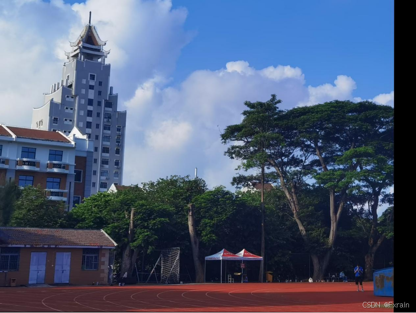
cv2.imwrite("D:/Computer vision/ransac_picture/drawMatchesBeforeRANSAC.jpg", drawImgBeforeRANSAC)(2)数据集(待拼接)

(3)实验结果截图
图3为输出的单应性矩阵结果截图:
如图所示,在运行SIFT特征检测和描述符提取后,通过BFMatcher进行特征匹配,初始匹配点的数量是198对。经过RANSAC算法去除错误匹配后,剩余的匹配点数量为1074对。这表明RANSAC算法有效地保留了正确的匹配点并去除了错误的匹配点。
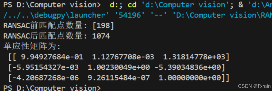
图4为在应用RANSAC算法之前绘制的匹配结果图像:
如图所示,绘制两幅图像的匹配结果并显示特征点之间的匹配关系。通过可视化匹配结果,可以直观地看到哪些特征点被成功匹配。
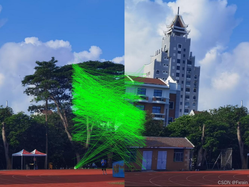
图5为最终拼接后的图像:
三、实验小结
图像拼接是计算机视觉领域的一个重要研究方向,通过将多张重叠的图像拼接在一起,实现更大、更全面的图像展示。实验中通过使用opencv中的相关函数实现图像的单应性变换,并使用BFMatcher和RANSAC算法进行了特征点匹配以及图像拼接。使用RANSAC算法后拼接效果良好,没有出现明显的错位或重叠问题。