当前位置：首页 > news >正文

【DGL】图分类

news 2025/7/1 16:41:56

概述

除了节点级别的问题——节点分类、边级别的问题——链接预测之外，还有整个图级别的问题——图分类。经过聚合、传递消息得到节点和边的新的表征后，映射得到整个图的表征。

数据集

dataset = dgl.data.GINDataset('PROTEINS', self_loop=True)
g = dataset[0]
print(g)
print("Node feature dimensionality:", dataset.dim_nfeats)
print("Number of graph categories:", dataset.gclasses)

(Graph(num_nodes=42, num_edges=204,ndata_schemes={'label': Scheme(shape=(), dtype=torch.int64), 'attr': Scheme(shape=(3,), dtype=torch.float32)}edata_schemes={}), tensor(0))
Node feature dimensionality: 3
Number of graph categories: 2

共1113个图，每个图中的节点的特征维度是3，图的类别数是2.

定义Data Loader

from torch.utils.data.sampler import SubsetRandomSamplerfrom dgl.dataloading import GraphDataLoadernum_examples = len(dataset)
num_train = int(num_examples * 0.8)train_sampler = SubsetRandomSampler(torch.arange(num_train))
test_sampler = SubsetRandomSampler(torch.arange(num_train, num_examples))train_dataloader = GraphDataLoader(dataset, sampler=train_sampler, batch_size=5, drop_last=False
)
test_dataloader = GraphDataLoader(dataset, sampler=test_sampler, batch_size=5, drop_last=False
)

取80%用作训练集，其余用作测试集
mini-batch操作，取5个graph打包成一个大的batched graph

it = iter(train_dataloader)
batch = next(it)
print(batch)

[Graph(num_nodes=259, num_edges=1201,ndata_schemes={'label': Scheme(shape=(), dtype=torch.int64), 'attr': Scheme(shape=(3,), dtype=torch.float32)}edata_schemes={}), tensor([0, 1, 0, 0, 0])]

DGL中的batched graph

在这里插入图片描述
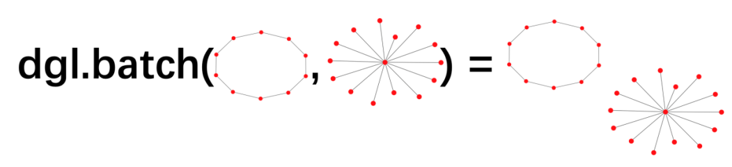
在每个mini-batch里面，batched graph是由dgl.batch对graph进行打包的

batched_graph, labels = batch
print("Number of nodes for each graph element in the batch:",batched_graph.batch_num_nodes(),
)
print("Number of edges for each graph element in the batch:",batched_graph.batch_num_edges(),
)# Recover the original graph elements from the minibatch
graphs = dgl.unbatch(batched_graph)
print("The original graphs in the minibatch:")
print(graphs)

Number of nodes for each graph element in the batch: tensor([ 55,  16, 116,  31,  41])
Number of edges for each graph element in the batch: tensor([209,  70, 584, 153, 185])
The original graphs in the minibatch:
[Graph(num_nodes=55, num_edges=209,ndata_schemes={'label': Scheme(shape=(), dtype=torch.int64), 'attr': Scheme(shape=(3,), dtype=torch.float32)}edata_schemes={}), Graph(num_nodes=16, num_edges=70,ndata_schemes={'label': Scheme(shape=(), dtype=torch.int64), 'attr': Scheme(shape=(3,), dtype=torch.float32)}edata_schemes={}), Graph(num_nodes=116, num_edges=584,ndata_schemes={'label': Scheme(shape=(), dtype=torch.int64), 'attr': Scheme(shape=(3,), dtype=torch.float32)}edata_schemes={}), Graph(num_nodes=31, num_edges=153,ndata_schemes={'label': Scheme(shape=(), dtype=torch.int64), 'attr': Scheme(shape=(3,), dtype=torch.float32)}edata_schemes={}), Graph(num_nodes=41, num_edges=185,ndata_schemes={'label': Scheme(shape=(), dtype=torch.int64), 'attr': Scheme(shape=(3,), dtype=torch.float32)}edata_schemes={})]

定义模型

class GCN(nn.Module):def __init__(self, in_feats, h_feats, num_classes):super(GCN, self).__init__()self.conv1 = GraphConv(in_feats, h_feats)self.conv2 = GraphConv(h_feats, num_classes)def forward(self, g, in_feat):h = self.conv1(g, in_feat)h = F.relu(h)h = self.conv2(g, h)g.ndata["h"] = hreturn dgl.mean_nodes(g, "h")#取所有节点的'h'特征的平均值来表征整个图  readoutmodel = GCN(dataset.dim_nfeats, 16, dataset.gclasses)
optimizer = torch.optim.Adam(model.parameters(), lr=0.01)

一个batched graph中，不同的图是完全分开的，即没有边连接两个图，所有消息传递函数仍然具有相同的结果（和没有打包之前相比）。
其次，将对每个图分别执行readout功能。假设批次大小为B，要聚合的特征维度为D，则读取出的形状为（B， D）。

训练

for epoch in range(20):num_correct = 0num_trains = 0for batched_graph, labels in train_dataloader:pred = model(batched_graph, batched_graph.ndata['attr'].float())loss = F.cross_entropy(pred, labels)num_trains += len(labels)num_correct += (pred.argmax(1)==labels).sum().item()optimizer.zero_grad()loss.backward()optimizer.step()print('train accuracy: ', num_correct/num_trains)num_correct = 0
num_tests = 0
for batched_graph, labels in test_dataloader:pred = model(batched_graph, batched_graph.ndata['attr'].float())num_correct += (pred.argmax(1)==labels).sum().item()num_tests += len(labels)print("Test accuracy: ", num_correct/num_tests)

train accuracy:  0.7404494382022472
train accuracy:  0.7426966292134831
train accuracy:  0.7471910112359551
train accuracy:  0.7539325842696629
train accuracy:  0.7584269662921348
train accuracy:  0.7674157303370787
train accuracy:  0.7629213483146068
train accuracy:  0.7617977528089888
train accuracy:  0.7584269662921348
train accuracy:  0.7707865168539326
train accuracy:  0.7629213483146068
train accuracy:  0.7651685393258427
train accuracy:  0.7629213483146068
train accuracy:  0.7561797752808989
train accuracy:  0.7606741573033707
train accuracy:  0.7584269662921348
train accuracy:  0.7617977528089888
train accuracy:  0.7707865168539326
train accuracy:  0.7629213483146068
train accuracy:  0.7539325842696629Test accuracy:  0.26905829596412556

效果非常一般明显过拟合应该和没有边特征，节点特征信息不足有关。