当前位置：首页 > news >正文

【Python机器学习】实验04(1) 多分类(基于逻辑回归)实践

news 2025/7/23 14:40:20

文章目录

多分类以及机器学习实践
- 如何对多个类别进行分类
- - 1.1 数据的预处理
  - 1.2 训练数据的准备
  - 1.3 定义假设函数，代价函数，梯度下降算法（从实验3复制过来）
  - 1.4 调用梯度下降算法来学习三个分类模型的参数
  - 1.5 利用模型进行预测
  - 1.6 评估模型
  - 1.7 试试sklearn
- 实验4(1) 请动手完成你们第一个多分类问题，祝好运！完成下面代码
- - 2.1 数据读取
  - 2.2 训练数据的准备
  - 2.3 定义假设函数、代价函数和梯度下降算法
  - 2.4 学习这四个分类模型
  - 2.5 利用模型进行预测
  - 2.6 计算准确率

多分类以及机器学习实践

如何对多个类别进行分类

Iris数据集是常用的分类实验数据集，由Fisher, 1936收集整理。Iris也称鸢尾花卉数据集，是一类多重变量分析的数据集。数据集包含150个数据样本，分为3类，每类50个数据，每个数据包含4个属性。可通过花萼长度，花萼宽度，花瓣长度，花瓣宽度4个属性预测鸢尾花卉属于（Setosa，Versicolour，Virginica）三个种类中的哪一类。

iris以鸢尾花的特征作为数据来源，常用在分类操作中。该数据集由3种不同类型的鸢尾花的各50个样本数据构成。其中的一个种类与另外两个种类是线性可分离的，后两个种类是非线性可分离的。

该数据集包含了4个属性：
Sepal.Length（花萼长度），单位是cm;
Sepal.Width（花萼宽度），单位是cm;
Petal.Length（花瓣长度），单位是cm;
Petal.Width（花瓣宽度），单位是cm;

种类：Iris Setosa（山鸢尾）、Iris Versicolour（杂色鸢尾），以及Iris Virginica（维吉尼亚鸢尾）。

1.1 数据的预处理

import sklearn.datasets as datasets
import pandas as pd
import numpy as np

data=datasets.load_iris()
data

{'data': array([[5.1, 3.5, 1.4, 0.2],[4.9, 3. , 1.4, 0.2],[4.7, 3.2, 1.3, 0.2],[4.6, 3.1, 1.5, 0.2],[5. , 3.6, 1.4, 0.2],[5.4, 3.9, 1.7, 0.4],[4.6, 3.4, 1.4, 0.3],[5. , 3.4, 1.5, 0.2],[4.4, 2.9, 1.4, 0.2],[4.9, 3.1, 1.5, 0.1],[5.4, 3.7, 1.5, 0.2],[4.8, 3.4, 1.6, 0.2],[4.8, 3. , 1.4, 0.1],[4.3, 3. , 1.1, 0.1],[5.8, 4. , 1.2, 0.2],[5.7, 4.4, 1.5, 0.4],[5.4, 3.9, 1.3, 0.4],[5.1, 3.5, 1.4, 0.3],[5.7, 3.8, 1.7, 0.3],[5.1, 3.8, 1.5, 0.3],[5.4, 3.4, 1.7, 0.2],[5.1, 3.7, 1.5, 0.4],[4.6, 3.6, 1. , 0.2],[5.1, 3.3, 1.7, 0.5],[4.8, 3.4, 1.9, 0.2],[5. , 3. , 1.6, 0.2],[5. , 3.4, 1.6, 0.4],[5.2, 3.5, 1.5, 0.2],[5.2, 3.4, 1.4, 0.2],[4.7, 3.2, 1.6, 0.2],[4.8, 3.1, 1.6, 0.2],[5.4, 3.4, 1.5, 0.4],[5.2, 4.1, 1.5, 0.1],[5.5, 4.2, 1.4, 0.2],[4.9, 3.1, 1.5, 0.2],[5. , 3.2, 1.2, 0.2],[5.5, 3.5, 1.3, 0.2],[4.9, 3.6, 1.4, 0.1],[4.4, 3. , 1.3, 0.2],[5.1, 3.4, 1.5, 0.2],[5. , 3.5, 1.3, 0.3],[4.5, 2.3, 1.3, 0.3],[4.4, 3.2, 1.3, 0.2],[5. , 3.5, 1.6, 0.6],[5.1, 3.8, 1.9, 0.4],[4.8, 3. , 1.4, 0.3],[5.1, 3.8, 1.6, 0.2],[4.6, 3.2, 1.4, 0.2],[5.3, 3.7, 1.5, 0.2],[5. , 3.3, 1.4, 0.2],[7. , 3.2, 4.7, 1.4],[6.4, 3.2, 4.5, 1.5],[6.9, 3.1, 4.9, 1.5],[5.5, 2.3, 4. , 1.3],[6.5, 2.8, 4.6, 1.5],[5.7, 2.8, 4.5, 1.3],[6.3, 3.3, 4.7, 1.6],[4.9, 2.4, 3.3, 1. ],[6.6, 2.9, 4.6, 1.3],[5.2, 2.7, 3.9, 1.4],[5. , 2. , 3.5, 1. ],[5.9, 3. , 4.2, 1.5],[6. , 2.2, 4. , 1. ],[6.1, 2.9, 4.7, 1.4],[5.6, 2.9, 3.6, 1.3],[6.7, 3.1, 4.4, 1.4],[5.6, 3. , 4.5, 1.5],[5.8, 2.7, 4.1, 1. ],[6.2, 2.2, 4.5, 1.5],[5.6, 2.5, 3.9, 1.1],[5.9, 3.2, 4.8, 1.8],[6.1, 2.8, 4. , 1.3],[6.3, 2.5, 4.9, 1.5],[6.1, 2.8, 4.7, 1.2],[6.4, 2.9, 4.3, 1.3],[6.6, 3. , 4.4, 1.4],[6.8, 2.8, 4.8, 1.4],[6.7, 3. , 5. , 1.7],[6. , 2.9, 4.5, 1.5],[5.7, 2.6, 3.5, 1. ],[5.5, 2.4, 3.8, 1.1],[5.5, 2.4, 3.7, 1. ],[5.8, 2.7, 3.9, 1.2],[6. , 2.7, 5.1, 1.6],[5.4, 3. , 4.5, 1.5],[6. , 3.4, 4.5, 1.6],[6.7, 3.1, 4.7, 1.5],[6.3, 2.3, 4.4, 1.3],[5.6, 3. , 4.1, 1.3],[5.5, 2.5, 4. , 1.3],[5.5, 2.6, 4.4, 1.2],[6.1, 3. , 4.6, 1.4],[5.8, 2.6, 4. , 1.2],[5. , 2.3, 3.3, 1. ],[5.6, 2.7, 4.2, 1.3],[5.7, 3. , 4.2, 1.2],[5.7, 2.9, 4.2, 1.3],[6.2, 2.9, 4.3, 1.3],[5.1, 2.5, 3. , 1.1],[5.7, 2.8, 4.1, 1.3],[6.3, 3.3, 6. , 2.5],[5.8, 2.7, 5.1, 1.9],[7.1, 3. , 5.9, 2.1],[6.3, 2.9, 5.6, 1.8],[6.5, 3. , 5.8, 2.2],[7.6, 3. , 6.6, 2.1],[4.9, 2.5, 4.5, 1.7],[7.3, 2.9, 6.3, 1.8],[6.7, 2.5, 5.8, 1.8],[7.2, 3.6, 6.1, 2.5],[6.5, 3.2, 5.1, 2. ],[6.4, 2.7, 5.3, 1.9],[6.8, 3. , 5.5, 2.1],[5.7, 2.5, 5. , 2. ],[5.8, 2.8, 5.1, 2.4],[6.4, 3.2, 5.3, 2.3],[6.5, 3. , 5.5, 1.8],[7.7, 3.8, 6.7, 2.2],[7.7, 2.6, 6.9, 2.3],[6. , 2.2, 5. , 1.5],[6.9, 3.2, 5.7, 2.3],[5.6, 2.8, 4.9, 2. ],[7.7, 2.8, 6.7, 2. ],[6.3, 2.7, 4.9, 1.8],[6.7, 3.3, 5.7, 2.1],[7.2, 3.2, 6. , 1.8],[6.2, 2.8, 4.8, 1.8],[6.1, 3. , 4.9, 1.8],[6.4, 2.8, 5.6, 2.1],[7.2, 3. , 5.8, 1.6],[7.4, 2.8, 6.1, 1.9],[7.9, 3.8, 6.4, 2. ],[6.4, 2.8, 5.6, 2.2],[6.3, 2.8, 5.1, 1.5],[6.1, 2.6, 5.6, 1.4],[7.7, 3. , 6.1, 2.3],[6.3, 3.4, 5.6, 2.4],[6.4, 3.1, 5.5, 1.8],[6. , 3. , 4.8, 1.8],[6.9, 3.1, 5.4, 2.1],[6.7, 3.1, 5.6, 2.4],[6.9, 3.1, 5.1, 2.3],[5.8, 2.7, 5.1, 1.9],[6.8, 3.2, 5.9, 2.3],[6.7, 3.3, 5.7, 2.5],[6.7, 3. , 5.2, 2.3],[6.3, 2.5, 5. , 1.9],[6.5, 3. , 5.2, 2. ],[6.2, 3.4, 5.4, 2.3],[5.9, 3. , 5.1, 1.8]]),'target': array([0, 0, 0, 0, 0, 0, 0, 0, 0, 0, 0, 0, 0, 0, 0, 0, 0, 0, 0, 0, 0, 0,0, 0, 0, 0, 0, 0, 0, 0, 0, 0, 0, 0, 0, 0, 0, 0, 0, 0, 0, 0, 0, 0,0, 0, 0, 0, 0, 0, 1, 1, 1, 1, 1, 1, 1, 1, 1, 1, 1, 1, 1, 1, 1, 1,1, 1, 1, 1, 1, 1, 1, 1, 1, 1, 1, 1, 1, 1, 1, 1, 1, 1, 1, 1, 1, 1,1, 1, 1, 1, 1, 1, 1, 1, 1, 1, 1, 1, 2, 2, 2, 2, 2, 2, 2, 2, 2, 2,2, 2, 2, 2, 2, 2, 2, 2, 2, 2, 2, 2, 2, 2, 2, 2, 2, 2, 2, 2, 2, 2,2, 2, 2, 2, 2, 2, 2, 2, 2, 2, 2, 2, 2, 2, 2, 2, 2, 2]),'frame': None,'target_names': array(['setosa', 'versicolor', 'virginica'], dtype='<U10'),'DESCR': '.. _iris_dataset:\n\nIris plants dataset\n--------------------\n\n**Data Set Characteristics:**\n\n    :Number of Instances: 150 (50 in each of three classes)\n    :Number of Attributes: 4 numeric, predictive attributes and the class\n    :Attribute Information:\n        - sepal length in cm\n        - sepal width in cm\n        - petal length in cm\n        - petal width in cm\n        - class:\n                - Iris-Setosa\n                - Iris-Versicolour\n                - Iris-Virginica\n                \n    :Summary Statistics:\n\n    ============== ==== ==== ======= ===== ====================\n                    Min  Max   Mean    SD   Class Correlation\n    ============== ==== ==== ======= ===== ====================\n    sepal length:   4.3  7.9   5.84   0.83    0.7826\n    sepal width:    2.0  4.4   3.05   0.43   -0.4194\n    petal length:   1.0  6.9   3.76   1.76    0.9490  (high!)\n    petal width:    0.1  2.5   1.20   0.76    0.9565  (high!)\n    ============== ==== ==== ======= ===== ====================\n\n    :Missing Attribute Values: None\n    :Class Distribution: 33.3% for each of 3 classes.\n    :Creator: R.A. Fisher\n    :Donor: Michael Marshall (MARSHALL%PLU@io.arc.nasa.gov)\n    :Date: July, 1988\n\nThe famous Iris database, first used by Sir R.A. Fisher. The dataset is taken\nfrom Fisher\'s paper. Note that it\'s the same as in R, but not as in the UCI\nMachine Learning Repository, which has two wrong data points.\n\nThis is perhaps the best known database to be found in the\npattern recognition literature.  Fisher\'s paper is a classic in the field and\nis referenced frequently to this day.  (See Duda & Hart, for example.)  The\ndata set contains 3 classes of 50 instances each, where each class refers to a\ntype of iris plant.  One class is linearly separable from the other 2; the\nlatter are NOT linearly separable from each other.\n\n.. topic:: References\n\n   - Fisher, R.A. "The use of multiple measurements in taxonomic problems"\n     Annual Eugenics, 7, Part II, 179-188 (1936); also in "Contributions to\n     Mathematical Statistics" (John Wiley, NY, 1950).\n   - Duda, R.O., & Hart, P.E. (1973) Pattern Classification and Scene Analysis.\n     (Q327.D83) John Wiley & Sons.  ISBN 0-471-22361-1.  See page 218.\n   - Dasarathy, B.V. (1980) "Nosing Around the Neighborhood: A New System\n     Structure and Classification Rule for Recognition in Partially Exposed\n     Environments".  IEEE Transactions on Pattern Analysis and Machine\n     Intelligence, Vol. PAMI-2, No. 1, 67-71.\n   - Gates, G.W. (1972) "The Reduced Nearest Neighbor Rule".  IEEE Transactions\n     on Information Theory, May 1972, 431-433.\n   - See also: 1988 MLC Proceedings, 54-64.  Cheeseman et al"s AUTOCLASS II\n     conceptual clustering system finds 3 classes in the data.\n   - Many, many more ...','feature_names': ['sepal length (cm)','sepal width (cm)','petal length (cm)','petal width (cm)'],'filename': 'iris.csv','data_module': 'sklearn.datasets.data'}

data_x=data["data"]
data_y=data["target"]

data_x.shape,data_y.shape

((150, 4), (150,))

data_y=data_y.reshape([len(data_y),1])
data_y

array([[0],[0],[0],[0],[0],[0],[0],[0],[0],[0],[0],[0],[0],[0],[0],[0],[0],[0],[0],[0],[0],[0],[0],[0],[0],[0],[0],[0],[0],[0],[0],[0],[0],[0],[0],[0],[0],[0],[0],[0],[0],[0],[0],[0],[0],[0],[0],[0],[0],[0],[1],[1],[1],[1],[1],[1],[1],[1],[1],[1],[1],[1],[1],[1],[1],[1],[1],[1],[1],[1],[1],[1],[1],[1],[1],[1],[1],[1],[1],[1],[1],[1],[1],[1],[1],[1],[1],[1],[1],[1],[1],[1],[1],[1],[1],[1],[1],[1],[1],[1],[2],[2],[2],[2],[2],[2],[2],[2],[2],[2],[2],[2],[2],[2],[2],[2],[2],[2],[2],[2],[2],[2],[2],[2],[2],[2],[2],[2],[2],[2],[2],[2],[2],[2],[2],[2],[2],[2],[2],[2],[2],[2],[2],[2],[2],[2],[2],[2],[2],[2]])

#法1 ，用拼接的方法
data=np.hstack([data_x,data_y])

#法二： 用插入的方法
np.insert(data_x,data_x.shape[1],data_y,axis=1)

array([[5.1, 3.5, 1.4, ..., 2. , 2. , 2. ],[4.9, 3. , 1.4, ..., 2. , 2. , 2. ],[4.7, 3.2, 1.3, ..., 2. , 2. , 2. ],...,[6.5, 3. , 5.2, ..., 2. , 2. , 2. ],[6.2, 3.4, 5.4, ..., 2. , 2. , 2. ],[5.9, 3. , 5.1, ..., 2. , 2. , 2. ]])

data=pd.DataFrame(data,columns=["F1","F2","F3","F4","target"])
data

	F1	F2	F3	F4	target
0	5.1	3.5	1.4	0.2	0.0
1	4.9	3.0	1.4	0.2	0.0
2	4.7	3.2	1.3	0.2	0.0
3	4.6	3.1	1.5	0.2	0.0
4	5.0	3.6	1.4	0.2	0.0
...	...	...	...	...	...
145	6.7	3.0	5.2	2.3	2.0
146	6.3	2.5	5.0	1.9	2.0
147	6.5	3.0	5.2	2.0	2.0
148	6.2	3.4	5.4	2.3	2.0
149	5.9	3.0	5.1	1.8	2.0

150 rows × 5 columns

data.insert(0,"ones",1)

data

	ones	F1	F2	F3	F4	target
0	1	5.1	3.5	1.4	0.2	0.0
1	1	4.9	3.0	1.4	0.2	0.0
2	1	4.7	3.2	1.3	0.2	0.0
3	1	4.6	3.1	1.5	0.2	0.0
4	1	5.0	3.6	1.4	0.2	0.0
...	...	...	...	...	...	...
145	1	6.7	3.0	5.2	2.3	2.0
146	1	6.3	2.5	5.0	1.9	2.0
147	1	6.5	3.0	5.2	2.0	2.0
148	1	6.2	3.4	5.4	2.3	2.0
149	1	5.9	3.0	5.1	1.8	2.0

150 rows × 6 columns

data["target"]=data["target"].astype("int32")

data

	ones	F1	F2	F3	F4	target
0	1	5.1	3.5	1.4	0.2	0
1	1	4.9	3.0	1.4	0.2	0
2	1	4.7	3.2	1.3	0.2	0
3	1	4.6	3.1	1.5	0.2	0
4	1	5.0	3.6	1.4	0.2	0
...	...	...	...	...	...	...
145	1	6.7	3.0	5.2	2.3	2
146	1	6.3	2.5	5.0	1.9	2
147	1	6.5	3.0	5.2	2.0	2
148	1	6.2	3.4	5.4	2.3	2
149	1	5.9	3.0	5.1	1.8	2

150 rows × 6 columns

1.2 训练数据的准备

data_x

array([[5.1, 3.5, 1.4, 0.2],[4.9, 3. , 1.4, 0.2],[4.7, 3.2, 1.3, 0.2],[4.6, 3.1, 1.5, 0.2],[5. , 3.6, 1.4, 0.2],[5.4, 3.9, 1.7, 0.4],[4.6, 3.4, 1.4, 0.3],[5. , 3.4, 1.5, 0.2],[4.4, 2.9, 1.4, 0.2],[4.9, 3.1, 1.5, 0.1],[5.4, 3.7, 1.5, 0.2],[4.8, 3.4, 1.6, 0.2],[4.8, 3. , 1.4, 0.1],[4.3, 3. , 1.1, 0.1],[5.8, 4. , 1.2, 0.2],[5.7, 4.4, 1.5, 0.4],[5.4, 3.9, 1.3, 0.4],[5.1, 3.5, 1.4, 0.3],[5.7, 3.8, 1.7, 0.3],[5.1, 3.8, 1.5, 0.3],[5.4, 3.4, 1.7, 0.2],[5.1, 3.7, 1.5, 0.4],[4.6, 3.6, 1. , 0.2],[5.1, 3.3, 1.7, 0.5],[4.8, 3.4, 1.9, 0.2],[5. , 3. , 1.6, 0.2],[5. , 3.4, 1.6, 0.4],[5.2, 3.5, 1.5, 0.2],[5.2, 3.4, 1.4, 0.2],[4.7, 3.2, 1.6, 0.2],[4.8, 3.1, 1.6, 0.2],[5.4, 3.4, 1.5, 0.4],[5.2, 4.1, 1.5, 0.1],[5.5, 4.2, 1.4, 0.2],[4.9, 3.1, 1.5, 0.2],[5. , 3.2, 1.2, 0.2],[5.5, 3.5, 1.3, 0.2],[4.9, 3.6, 1.4, 0.1],[4.4, 3. , 1.3, 0.2],[5.1, 3.4, 1.5, 0.2],[5. , 3.5, 1.3, 0.3],[4.5, 2.3, 1.3, 0.3],[4.4, 3.2, 1.3, 0.2],[5. , 3.5, 1.6, 0.6],[5.1, 3.8, 1.9, 0.4],[4.8, 3. , 1.4, 0.3],[5.1, 3.8, 1.6, 0.2],[4.6, 3.2, 1.4, 0.2],[5.3, 3.7, 1.5, 0.2],[5. , 3.3, 1.4, 0.2],[7. , 3.2, 4.7, 1.4],[6.4, 3.2, 4.5, 1.5],[6.9, 3.1, 4.9, 1.5],[5.5, 2.3, 4. , 1.3],[6.5, 2.8, 4.6, 1.5],[5.7, 2.8, 4.5, 1.3],[6.3, 3.3, 4.7, 1.6],[4.9, 2.4, 3.3, 1. ],[6.6, 2.9, 4.6, 1.3],[5.2, 2.7, 3.9, 1.4],[5. , 2. , 3.5, 1. ],[5.9, 3. , 4.2, 1.5],[6. , 2.2, 4. , 1. ],[6.1, 2.9, 4.7, 1.4],[5.6, 2.9, 3.6, 1.3],[6.7, 3.1, 4.4, 1.4],[5.6, 3. , 4.5, 1.5],[5.8, 2.7, 4.1, 1. ],[6.2, 2.2, 4.5, 1.5],[5.6, 2.5, 3.9, 1.1],[5.9, 3.2, 4.8, 1.8],[6.1, 2.8, 4. , 1.3],[6.3, 2.5, 4.9, 1.5],[6.1, 2.8, 4.7, 1.2],[6.4, 2.9, 4.3, 1.3],[6.6, 3. , 4.4, 1.4],[6.8, 2.8, 4.8, 1.4],[6.7, 3. , 5. , 1.7],[6. , 2.9, 4.5, 1.5],[5.7, 2.6, 3.5, 1. ],[5.5, 2.4, 3.8, 1.1],[5.5, 2.4, 3.7, 1. ],[5.8, 2.7, 3.9, 1.2],[6. , 2.7, 5.1, 1.6],[5.4, 3. , 4.5, 1.5],[6. , 3.4, 4.5, 1.6],[6.7, 3.1, 4.7, 1.5],[6.3, 2.3, 4.4, 1.3],[5.6, 3. , 4.1, 1.3],[5.5, 2.5, 4. , 1.3],[5.5, 2.6, 4.4, 1.2],[6.1, 3. , 4.6, 1.4],[5.8, 2.6, 4. , 1.2],[5. , 2.3, 3.3, 1. ],[5.6, 2.7, 4.2, 1.3],[5.7, 3. , 4.2, 1.2],[5.7, 2.9, 4.2, 1.3],[6.2, 2.9, 4.3, 1.3],[5.1, 2.5, 3. , 1.1],[5.7, 2.8, 4.1, 1.3],[6.3, 3.3, 6. , 2.5],[5.8, 2.7, 5.1, 1.9],[7.1, 3. , 5.9, 2.1],[6.3, 2.9, 5.6, 1.8],[6.5, 3. , 5.8, 2.2],[7.6, 3. , 6.6, 2.1],[4.9, 2.5, 4.5, 1.7],[7.3, 2.9, 6.3, 1.8],[6.7, 2.5, 5.8, 1.8],[7.2, 3.6, 6.1, 2.5],[6.5, 3.2, 5.1, 2. ],[6.4, 2.7, 5.3, 1.9],[6.8, 3. , 5.5, 2.1],[5.7, 2.5, 5. , 2. ],[5.8, 2.8, 5.1, 2.4],[6.4, 3.2, 5.3, 2.3],[6.5, 3. , 5.5, 1.8],[7.7, 3.8, 6.7, 2.2],[7.7, 2.6, 6.9, 2.3],[6. , 2.2, 5. , 1.5],[6.9, 3.2, 5.7, 2.3],[5.6, 2.8, 4.9, 2. ],[7.7, 2.8, 6.7, 2. ],[6.3, 2.7, 4.9, 1.8],[6.7, 3.3, 5.7, 2.1],[7.2, 3.2, 6. , 1.8],[6.2, 2.8, 4.8, 1.8],[6.1, 3. , 4.9, 1.8],[6.4, 2.8, 5.6, 2.1],[7.2, 3. , 5.8, 1.6],[7.4, 2.8, 6.1, 1.9],[7.9, 3.8, 6.4, 2. ],[6.4, 2.8, 5.6, 2.2],[6.3, 2.8, 5.1, 1.5],[6.1, 2.6, 5.6, 1.4],[7.7, 3. , 6.1, 2.3],[6.3, 3.4, 5.6, 2.4],[6.4, 3.1, 5.5, 1.8],[6. , 3. , 4.8, 1.8],[6.9, 3.1, 5.4, 2.1],[6.7, 3.1, 5.6, 2.4],[6.9, 3.1, 5.1, 2.3],[5.8, 2.7, 5.1, 1.9],[6.8, 3.2, 5.9, 2.3],[6.7, 3.3, 5.7, 2.5],[6.7, 3. , 5.2, 2.3],[6.3, 2.5, 5. , 1.9],[6.5, 3. , 5.2, 2. ],[6.2, 3.4, 5.4, 2.3],[5.9, 3. , 5.1, 1.8]])

data_x=np.insert(data_x,0,1,axis=1)

data_x.shape,data_y.shape

((150, 5), (150, 1))

#训练数据的特征和标签
data_x,data_y

(array([[1. , 5.1, 3.5, 1.4, 0.2],[1. , 4.9, 3. , 1.4, 0.2],[1. , 4.7, 3.2, 1.3, 0.2],[1. , 4.6, 3.1, 1.5, 0.2],[1. , 5. , 3.6, 1.4, 0.2],[1. , 5.4, 3.9, 1.7, 0.4],[1. , 4.6, 3.4, 1.4, 0.3],[1. , 5. , 3.4, 1.5, 0.2],[1. , 4.4, 2.9, 1.4, 0.2],[1. , 4.9, 3.1, 1.5, 0.1],[1. , 5.4, 3.7, 1.5, 0.2],[1. , 4.8, 3.4, 1.6, 0.2],[1. , 4.8, 3. , 1.4, 0.1],[1. , 4.3, 3. , 1.1, 0.1],[1. , 5.8, 4. , 1.2, 0.2],[1. , 5.7, 4.4, 1.5, 0.4],[1. , 5.4, 3.9, 1.3, 0.4],[1. , 5.1, 3.5, 1.4, 0.3],[1. , 5.7, 3.8, 1.7, 0.3],[1. , 5.1, 3.8, 1.5, 0.3],[1. , 5.4, 3.4, 1.7, 0.2],[1. , 5.1, 3.7, 1.5, 0.4],[1. , 4.6, 3.6, 1. , 0.2],[1. , 5.1, 3.3, 1.7, 0.5],[1. , 4.8, 3.4, 1.9, 0.2],[1. , 5. , 3. , 1.6, 0.2],[1. , 5. , 3.4, 1.6, 0.4],[1. , 5.2, 3.5, 1.5, 0.2],[1. , 5.2, 3.4, 1.4, 0.2],[1. , 4.7, 3.2, 1.6, 0.2],[1. , 4.8, 3.1, 1.6, 0.2],[1. , 5.4, 3.4, 1.5, 0.4],[1. , 5.2, 4.1, 1.5, 0.1],[1. , 5.5, 4.2, 1.4, 0.2],[1. , 4.9, 3.1, 1.5, 0.2],[1. , 5. , 3.2, 1.2, 0.2],[1. , 5.5, 3.5, 1.3, 0.2],[1. , 4.9, 3.6, 1.4, 0.1],[1. , 4.4, 3. , 1.3, 0.2],[1. , 5.1, 3.4, 1.5, 0.2],[1. , 5. , 3.5, 1.3, 0.3],[1. , 4.5, 2.3, 1.3, 0.3],[1. , 4.4, 3.2, 1.3, 0.2],[1. , 5. , 3.5, 1.6, 0.6],[1. , 5.1, 3.8, 1.9, 0.4],[1. , 4.8, 3. , 1.4, 0.3],[1. , 5.1, 3.8, 1.6, 0.2],[1. , 4.6, 3.2, 1.4, 0.2],[1. , 5.3, 3.7, 1.5, 0.2],[1. , 5. , 3.3, 1.4, 0.2],[1. , 7. , 3.2, 4.7, 1.4],[1. , 6.4, 3.2, 4.5, 1.5],[1. , 6.9, 3.1, 4.9, 1.5],[1. , 5.5, 2.3, 4. , 1.3],[1. , 6.5, 2.8, 4.6, 1.5],[1. , 5.7, 2.8, 4.5, 1.3],[1. , 6.3, 3.3, 4.7, 1.6],[1. , 4.9, 2.4, 3.3, 1. ],[1. , 6.6, 2.9, 4.6, 1.3],[1. , 5.2, 2.7, 3.9, 1.4],[1. , 5. , 2. , 3.5, 1. ],[1. , 5.9, 3. , 4.2, 1.5],[1. , 6. , 2.2, 4. , 1. ],[1. , 6.1, 2.9, 4.7, 1.4],[1. , 5.6, 2.9, 3.6, 1.3],[1. , 6.7, 3.1, 4.4, 1.4],[1. , 5.6, 3. , 4.5, 1.5],[1. , 5.8, 2.7, 4.1, 1. ],[1. , 6.2, 2.2, 4.5, 1.5],[1. , 5.6, 2.5, 3.9, 1.1],[1. , 5.9, 3.2, 4.8, 1.8],[1. , 6.1, 2.8, 4. , 1.3],[1. , 6.3, 2.5, 4.9, 1.5],[1. , 6.1, 2.8, 4.7, 1.2],[1. , 6.4, 2.9, 4.3, 1.3],[1. , 6.6, 3. , 4.4, 1.4],[1. , 6.8, 2.8, 4.8, 1.4],[1. , 6.7, 3. , 5. , 1.7],[1. , 6. , 2.9, 4.5, 1.5],[1. , 5.7, 2.6, 3.5, 1. ],[1. , 5.5, 2.4, 3.8, 1.1],[1. , 5.5, 2.4, 3.7, 1. ],[1. , 5.8, 2.7, 3.9, 1.2],[1. , 6. , 2.7, 5.1, 1.6],[1. , 5.4, 3. , 4.5, 1.5],[1. , 6. , 3.4, 4.5, 1.6],[1. , 6.7, 3.1, 4.7, 1.5],[1. , 6.3, 2.3, 4.4, 1.3],[1. , 5.6, 3. , 4.1, 1.3],[1. , 5.5, 2.5, 4. , 1.3],[1. , 5.5, 2.6, 4.4, 1.2],[1. , 6.1, 3. , 4.6, 1.4],[1. , 5.8, 2.6, 4. , 1.2],[1. , 5. , 2.3, 3.3, 1. ],[1. , 5.6, 2.7, 4.2, 1.3],[1. , 5.7, 3. , 4.2, 1.2],[1. , 5.7, 2.9, 4.2, 1.3],[1. , 6.2, 2.9, 4.3, 1.3],[1. , 5.1, 2.5, 3. , 1.1],[1. , 5.7, 2.8, 4.1, 1.3],[1. , 6.3, 3.3, 6. , 2.5],[1. , 5.8, 2.7, 5.1, 1.9],[1. , 7.1, 3. , 5.9, 2.1],[1. , 6.3, 2.9, 5.6, 1.8],[1. , 6.5, 3. , 5.8, 2.2],[1. , 7.6, 3. , 6.6, 2.1],[1. , 4.9, 2.5, 4.5, 1.7],[1. , 7.3, 2.9, 6.3, 1.8],[1. , 6.7, 2.5, 5.8, 1.8],[1. , 7.2, 3.6, 6.1, 2.5],[1. , 6.5, 3.2, 5.1, 2. ],[1. , 6.4, 2.7, 5.3, 1.9],[1. , 6.8, 3. , 5.5, 2.1],[1. , 5.7, 2.5, 5. , 2. ],[1. , 5.8, 2.8, 5.1, 2.4],[1. , 6.4, 3.2, 5.3, 2.3],[1. , 6.5, 3. , 5.5, 1.8],[1. , 7.7, 3.8, 6.7, 2.2],[1. , 7.7, 2.6, 6.9, 2.3],[1. , 6. , 2.2, 5. , 1.5],[1. , 6.9, 3.2, 5.7, 2.3],[1. , 5.6, 2.8, 4.9, 2. ],[1. , 7.7, 2.8, 6.7, 2. ],[1. , 6.3, 2.7, 4.9, 1.8],[1. , 6.7, 3.3, 5.7, 2.1],[1. , 7.2, 3.2, 6. , 1.8],[1. , 6.2, 2.8, 4.8, 1.8],[1. , 6.1, 3. , 4.9, 1.8],[1. , 6.4, 2.8, 5.6, 2.1],[1. , 7.2, 3. , 5.8, 1.6],[1. , 7.4, 2.8, 6.1, 1.9],[1. , 7.9, 3.8, 6.4, 2. ],[1. , 6.4, 2.8, 5.6, 2.2],[1. , 6.3, 2.8, 5.1, 1.5],[1. , 6.1, 2.6, 5.6, 1.4],[1. , 7.7, 3. , 6.1, 2.3],[1. , 6.3, 3.4, 5.6, 2.4],[1. , 6.4, 3.1, 5.5, 1.8],[1. , 6. , 3. , 4.8, 1.8],[1. , 6.9, 3.1, 5.4, 2.1],[1. , 6.7, 3.1, 5.6, 2.4],[1. , 6.9, 3.1, 5.1, 2.3],[1. , 5.8, 2.7, 5.1, 1.9],[1. , 6.8, 3.2, 5.9, 2.3],[1. , 6.7, 3.3, 5.7, 2.5],[1. , 6.7, 3. , 5.2, 2.3],[1. , 6.3, 2.5, 5. , 1.9],[1. , 6.5, 3. , 5.2, 2. ],[1. , 6.2, 3.4, 5.4, 2.3],[1. , 5.9, 3. , 5.1, 1.8]]),array([[0],[0],[0],[0],[0],[0],[0],[0],[0],[0],[0],[0],[0],[0],[0],[0],[0],[0],[0],[0],[0],[0],[0],[0],[0],[0],[0],[0],[0],[0],[0],[0],[0],[0],[0],[0],[0],[0],[0],[0],[0],[0],[0],[0],[0],[0],[0],[0],[0],[0],[1],[1],[1],[1],[1],[1],[1],[1],[1],[1],[1],[1],[1],[1],[1],[1],[1],[1],[1],[1],[1],[1],[1],[1],[1],[1],[1],[1],[1],[1],[1],[1],[1],[1],[1],[1],[1],[1],[1],[1],[1],[1],[1],[1],[1],[1],[1],[1],[1],[1],[2],[2],[2],[2],[2],[2],[2],[2],[2],[2],[2],[2],[2],[2],[2],[2],[2],[2],[2],[2],[2],[2],[2],[2],[2],[2],[2],[2],[2],[2],[2],[2],[2],[2],[2],[2],[2],[2],[2],[2],[2],[2],[2],[2],[2],[2],[2],[2],[2],[2]]))

由于有三个类别，那么在训练时三类数据要分开

data1=data.copy()

data1

	ones	F1	F2	F3	F4	target
0	1	5.1	3.5	1.4	0.2	0
1	1	4.9	3.0	1.4	0.2	0
2	1	4.7	3.2	1.3	0.2	0
3	1	4.6	3.1	1.5	0.2	0
4	1	5.0	3.6	1.4	0.2	0
...	...	...	...	...	...	...
145	1	6.7	3.0	5.2	2.3	2
146	1	6.3	2.5	5.0	1.9	2
147	1	6.5	3.0	5.2	2.0	2
148	1	6.2	3.4	5.4	2.3	2
149	1	5.9	3.0	5.1	1.8	2

150 rows × 6 columns

data

data1.loc[data["target"]!=0,"target"]=0
data1.loc[data["target"]==0,"target"]=1

data1

	ones	F1	F2	F3	F4	target
0	1	5.1	3.5	1.4	0.2	1
1	1	4.9	3.0	1.4	0.2	1
2	1	4.7	3.2	1.3	0.2	1
3	1	4.6	3.1	1.5	0.2	1
4	1	5.0	3.6	1.4	0.2	1
...	...	...	...	...	...	...
145	1	6.7	3.0	5.2	2.3	0
146	1	6.3	2.5	5.0	1.9	0
147	1	6.5	3.0	5.2	2.0	0
148	1	6.2	3.4	5.4	2.3	0
149	1	5.9	3.0	5.1	1.8	0

150 rows × 6 columns

data1_x=data1.iloc[:,:data1.shape[1]-1].values
data1_y=data1.iloc[:,data1.shape[1]-1].values
data1_x.shape,data1_y.shape

((150, 5), (150,))

#针对第二类，即第二个分类器的数据
data2=data.copy()
data2.loc[data["target"]==1,"target"]=1
data2.loc[data["target"]!=1,"target"]=0
data2["target"]==0

0      True
1      True
2      True
3      True
4      True... 
145    True
146    True
147    True
148    True
149    True
Name: target, Length: 150, dtype: bool

data2.shape[1]

data2.iloc[50:55,:]

	ones	F1	F2	F3	F4	target
50	1	7.0	3.2	4.7	1.4	1
51	1	6.4	3.2	4.5	1.5	1
52	1	6.9	3.1	4.9	1.5	1
53	1	5.5	2.3	4.0	1.3	1
54	1	6.5	2.8	4.6	1.5	1

data2_x=data2.iloc[:,:data2.shape[1]-1].values
data2_y=data2.iloc[:,data2.shape[1]-1].values

#针对第三类，即第三个分类器的数据
data3=data.copy()
data3.loc[data["target"]==2,"target"]=1
data3.loc[data["target"]!=2,"target"]=0
data3

	ones	F1	F2	F3	F4	target
0	1	5.1	3.5	1.4	0.2	0
1	1	4.9	3.0	1.4	0.2	0
2	1	4.7	3.2	1.3	0.2	0
3	1	4.6	3.1	1.5	0.2	0
4	1	5.0	3.6	1.4	0.2	0
...	...	...	...	...	...	...
145	1	6.7	3.0	5.2	2.3	1
146	1	6.3	2.5	5.0	1.9	1
147	1	6.5	3.0	5.2	2.0	1
148	1	6.2	3.4	5.4	2.3	1
149	1	5.9	3.0	5.1	1.8	1

150 rows × 6 columns

data3_x=data3.iloc[:,:data3.shape[1]-1].values
data3_y=data3.iloc[:,data3.shape[1]-1].values

1.3 定义假设函数，代价函数，梯度下降算法（从实验3复制过来）

def sigmoid(z):return 1 / (1 + np.exp(-z))

def h(X,w):z=X@wh=sigmoid(z)return h

#代价函数构造
def cost(X,w,y):#当X(m,n+1),y(m,),w(n+1,1)y_hat=sigmoid(X@w)right=np.multiply(y.ravel(),np.log(y_hat).ravel())+np.multiply((1-y).ravel(),np.log(1-y_hat).ravel())cost=-np.sum(right)/X.shape[0]return cost

def sigmoid(z):return 1 / (1 + np.exp(-z))def h(X,w):z=X@wh=sigmoid(z)return h#代价函数构造
def cost(X,w,y):#当X(m,n+1),y(m,),w(n+1,1)y_hat=sigmoid(X@w)right=np.multiply(y.ravel(),np.log(y_hat).ravel())+np.multiply((1-y).ravel(),np.log(1-y_hat).ravel())cost=-np.sum(right)/X.shape[0]return costdef grandient(X,y,iter_num,alpha):y=y.reshape((X.shape[0],1))w=np.zeros((X.shape[1],1))cost_lst=[]  for i in range(iter_num):y_pred=h(X,w)-ytemp=np.zeros((X.shape[1],1))for j in range(X.shape[1]):right=np.multiply(y_pred.ravel(),X[:,j])gradient=1/(X.shape[0])*(np.sum(right))temp[j,0]=w[j,0]-alpha*gradientw=tempcost_lst.append(cost(X,w,y.ravel()))return w,cost_lst

1.4 调用梯度下降算法来学习三个分类模型的参数

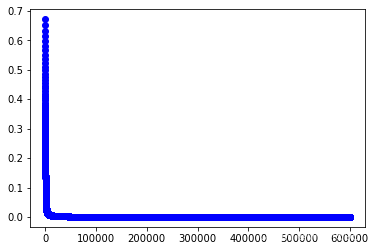
#初始化超参数
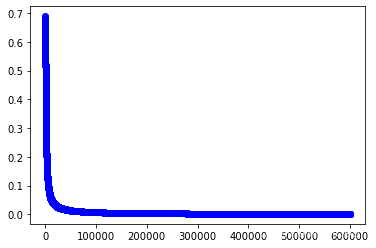
iter_num,alpha=600000,0.001

#训练第一个模型
w1,cost_lst1=grandient(data1_x,data1_y,iter_num,alpha)

import matplotlib.pyplot as plt
plt.plot(range(iter_num),cost_lst1,"b-o")

[<matplotlib.lines.Line2D at 0x2562630b100>]

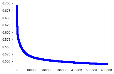
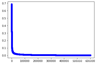
#训练第二个模型
w2,cost_lst2=grandient(data2_x,data2_y,iter_num,alpha)

import matplotlib.pyplot as plt
plt.plot(range(iter_num),cost_lst2,"b-o")

[<matplotlib.lines.Line2D at 0x25628114280>]

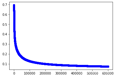
#训练第三个模型
w3,cost_lst3=grandient(data3_x,data3_y,iter_num,alpha)

w3

array([[-3.22437049],[-3.50214058],[-3.50286355],[ 5.16580317],[ 5.89898368]])

import matplotlib.pyplot as plt
plt.plot(range(iter_num),cost_lst3,"b-o")

[<matplotlib.lines.Line2D at 0x2562e0f81c0>]

1.5 利用模型进行预测

h(data_x,w3)

array([[1.48445441e-11],[1.72343968e-10],[1.02798153e-10],[5.81975546e-10],[1.48434710e-11],[1.95971176e-11],[2.18959639e-10],[5.01346874e-11],[1.40930075e-09],[1.12830635e-10],[4.31888744e-12],[1.69308343e-10],[1.35613372e-10],[1.65858883e-10],[7.89880725e-14],[4.23224675e-13],[2.48199140e-12],[2.67766642e-11],[5.39314286e-12],[1.56935848e-11],[3.47096426e-11],[4.01827075e-11],[7.63005509e-12],[8.26864773e-10],[7.97484594e-10],[3.41189783e-10],[2.73442178e-10],[1.75314894e-11],[1.48456174e-11],[4.84204982e-10],[4.84239990e-10],[4.01914238e-11],[1.18813180e-12],[3.14985611e-13],[2.03524473e-10],[2.14461446e-11],[2.18189955e-12],[1.16799745e-11],[5.92281641e-10],[3.53217554e-11],[2.26727669e-11],[8.74004884e-09],[2.93949962e-10],[6.26783110e-10],[2.23513465e-10],[4.41246960e-10],[1.45841303e-11],[2.44584721e-10],[6.13010507e-12],[4.24539165e-11],[1.64123143e-03],[8.55503211e-03],[1.65105645e-02],[9.87814122e-02],[3.97290777e-02],[1.11076040e-01],[4.19003715e-02],[2.88426221e-03],[6.27161978e-03],[7.67020481e-02],[2.27204861e-02],[2.08212169e-02],[4.58067633e-03],[9.90450665e-02],[1.19419048e-03],[1.41462060e-03],[2.22638069e-01],[2.68940904e-03],[3.66014737e-01],[6.97791873e-03],[5.78803255e-01],[2.32071970e-03],[5.28941621e-01],[4.57649874e-02],[2.69208900e-03],[2.84603646e-03],[2.20421076e-02],[2.07507605e-01],[9.10460936e-02],[2.44824946e-04],[8.37509821e-03],[2.78543808e-03],[3.11283202e-03],[8.89831833e-01],[3.65880536e-01],[3.03993844e-02],[1.18930239e-02],[4.99150151e-02],[1.10252946e-02],[5.15923462e-02],[1.43653056e-01],[4.41610209e-02],[7.37513950e-03],[2.88447014e-03],[5.07366744e-02],[7.24617687e-03],[1.83460602e-02],[5.40874928e-03],[3.87210511e-04],[1.55791816e-02],[9.99862942e-01],[9.89637526e-01],[9.86183040e-01],[9.83705644e-01],[9.98410187e-01],[9.97834502e-01],[9.84208537e-01],[9.85434538e-01],[9.94141336e-01],[9.94561329e-01],[7.20333384e-01],[9.70431293e-01],[9.62754456e-01],[9.96609064e-01],[9.99222270e-01],[9.83684437e-01],[9.26437633e-01],[9.83486260e-01],[9.99950496e-01],[9.39002061e-01],[9.88043323e-01],[9.88637702e-01],[9.98357641e-01],[7.65848930e-01],[9.73006160e-01],[8.76969899e-01],[6.61137141e-01],[6.97324053e-01],[9.97185846e-01],[6.11033594e-01],[9.77494647e-01],[6.58573810e-01],[9.98437920e-01],[5.24529693e-01],[9.70465066e-01],[9.87624920e-01],[9.97236435e-01],[9.26432706e-01],[6.61104746e-01],[8.84442100e-01],[9.96082862e-01],[8.40940308e-01],[9.89637526e-01],[9.96974990e-01],[9.97386310e-01],[9.62040470e-01],[9.52214579e-01],[8.96902215e-01],[9.90200940e-01],[9.28785160e-01]])

#将数据输入三个模型的看看结果
multi_pred=pd.DataFrame(zip(h(data_x,w1).ravel(),h(data_x,w2).ravel(),h(data_x,w3).ravel()))
multi_pred

	0	1	2
0	0.999297	0.108037	1.484454e-11
1	0.997061	0.270814	1.723440e-10
2	0.998633	0.164710	1.027982e-10
3	0.995774	0.231910	5.819755e-10
4	0.999415	0.085259	1.484347e-11
...	...	...	...
145	0.000007	0.127574	9.620405e-01
146	0.000006	0.496389	9.522146e-01
147	0.000010	0.234745	8.969022e-01
148	0.000006	0.058444	9.902009e-01
149	0.000014	0.284295	9.287852e-01

150 rows × 3 columns

multi_pred.values[:3]

array([[9.99297209e-01, 1.08037473e-01, 1.48445441e-11],[9.97060801e-01, 2.70813780e-01, 1.72343968e-10],[9.98632728e-01, 1.64709623e-01, 1.02798153e-10]])

#每个样本的预测值
np.argmax(multi_pred.values,axis=1)

array([0, 0, 0, 0, 0, 0, 0, 0, 0, 0, 0, 0, 0, 0, 0, 0, 0, 0, 0, 0, 0, 0,0, 0, 0, 0, 0, 0, 0, 0, 0, 0, 0, 0, 0, 0, 0, 0, 0, 0, 0, 0, 0, 0,0, 0, 0, 0, 0, 0, 1, 1, 1, 1, 1, 1, 1, 1, 1, 1, 1, 1, 1, 1, 1, 1,1, 1, 1, 1, 2, 1, 1, 1, 1, 1, 1, 1, 1, 1, 1, 1, 1, 2, 2, 1, 1, 1,1, 1, 1, 1, 1, 1, 1, 1, 1, 1, 1, 1, 2, 2, 2, 2, 2, 2, 2, 2, 2, 2,2, 2, 2, 2, 2, 2, 2, 2, 2, 2, 2, 2, 2, 2, 2, 2, 2, 2, 2, 1, 2, 2,2, 1, 2, 2, 2, 2, 2, 2, 2, 2, 2, 2, 2, 2, 2, 2, 2, 2], dtype=int64)

#每个样本的真实值
data_y

array([[0],[0],[0],[0],[0],[0],[0],[0],[0],[0],[0],[0],[0],[0],[0],[0],[0],[0],[0],[0],[0],[0],[0],[0],[0],[0],[0],[0],[0],[0],[0],[0],[0],[0],[0],[0],[0],[0],[0],[0],[0],[0],[0],[0],[0],[0],[0],[0],[0],[0],[1],[1],[1],[1],[1],[1],[1],[1],[1],[1],[1],[1],[1],[1],[1],[1],[1],[1],[1],[1],[1],[1],[1],[1],[1],[1],[1],[1],[1],[1],[1],[1],[1],[1],[1],[1],[1],[1],[1],[1],[1],[1],[1],[1],[1],[1],[1],[1],[1],[1],[2],[2],[2],[2],[2],[2],[2],[2],[2],[2],[2],[2],[2],[2],[2],[2],[2],[2],[2],[2],[2],[2],[2],[2],[2],[2],[2],[2],[2],[2],[2],[2],[2],[2],[2],[2],[2],[2],[2],[2],[2],[2],[2],[2],[2],[2],[2],[2],[2],[2]])

1.6 评估模型

np.argmax(multi_pred.values,axis=1)==data_y.ravel()

array([ True,  True,  True,  True,  True,  True,  True,  True,  True,True,  True,  True,  True,  True,  True,  True,  True,  True,True,  True,  True,  True,  True,  True,  True,  True,  True,True,  True,  True,  True,  True,  True,  True,  True,  True,True,  True,  True,  True,  True,  True,  True,  True,  True,True,  True,  True,  True,  True,  True,  True,  True,  True,True,  True,  True,  True,  True,  True,  True,  True,  True,True,  True,  True,  True,  True,  True,  True, False,  True,True,  True,  True,  True,  True,  True,  True,  True,  True,True,  True, False, False,  True,  True,  True,  True,  True,True,  True,  True,  True,  True,  True,  True,  True,  True,True,  True,  True,  True,  True,  True,  True,  True,  True,True,  True,  True,  True,  True,  True,  True,  True,  True,True,  True,  True,  True,  True,  True,  True,  True,  True,True,  True,  True, False,  True,  True,  True, False,  True,True,  True,  True,  True,  True,  True,  True,  True,  True,True,  True,  True,  True,  True,  True])

np.sum(np.argmax(multi_pred.values,axis=1)==data_y.ravel())

np.sum(np.argmax(multi_pred.values,axis=1)==data_y.ravel())/len(data)

0.9666666666666667

1.7 试试sklearn

from sklearn.linear_model import LogisticRegression
#建立第一个模型
clf1=LogisticRegression()
clf1.fit(data1_x,data1_y)
#建立第二个模型
clf2=LogisticRegression()
clf2.fit(data2_x,data2_y)
#建立第三个模型
clf3=LogisticRegression()
clf3.fit(data3_x,data3_y)

LogisticRegression()

y_pred1=clf1.predict(data_x)
y_pred2=clf2.predict(data_x)
y_pred3=clf3.predict(data_x)

#可视化各模型的预测结果
multi_pred=pd.DataFrame(zip(y_pred1,y_pred2,y_pred3),columns=["模型1","模糊2","模型3"])
multi_pred

	模型1	模糊2	模型3
0	1	0	0
1	1	0	0
2	1	0	0
3	1	0	0
4	1	0	0
...	...	...	...
145	0	0	1
146	0	1	1
147	0	0	1
148	0	0	1
149	0	0	1

150 rows × 3 columns

#判断预测结果
np.argmax(multi_pred.values,axis=1)

array([0, 0, 0, 0, 0, 0, 0, 0, 0, 0, 0, 0, 0, 0, 0, 0, 0, 0, 0, 0, 0, 0,0, 0, 0, 0, 0, 0, 0, 0, 0, 0, 0, 0, 0, 0, 0, 0, 0, 0, 0, 0, 0, 0,0, 0, 0, 0, 0, 0, 0, 0, 0, 1, 0, 1, 0, 1, 0, 0, 1, 0, 1, 0, 0, 0,0, 1, 1, 1, 2, 0, 1, 1, 0, 0, 0, 2, 0, 1, 1, 1, 0, 1, 0, 0, 0, 1,0, 1, 1, 0, 1, 1, 1, 0, 0, 0, 1, 0, 2, 2, 2, 2, 2, 2, 1, 1, 1, 2,2, 2, 2, 1, 2, 2, 2, 2, 1, 1, 2, 2, 1, 2, 2, 2, 2, 2, 2, 2, 1, 2,2, 1, 1, 2, 2, 2, 2, 2, 2, 2, 2, 2, 2, 2, 1, 2, 2, 2], dtype=int64)

data_y.ravel()

array([0, 0, 0, 0, 0, 0, 0, 0, 0, 0, 0, 0, 0, 0, 0, 0, 0, 0, 0, 0, 0, 0,0, 0, 0, 0, 0, 0, 0, 0, 0, 0, 0, 0, 0, 0, 0, 0, 0, 0, 0, 0, 0, 0,0, 0, 0, 0, 0, 0, 1, 1, 1, 1, 1, 1, 1, 1, 1, 1, 1, 1, 1, 1, 1, 1,1, 1, 1, 1, 1, 1, 1, 1, 1, 1, 1, 1, 1, 1, 1, 1, 1, 1, 1, 1, 1, 1,1, 1, 1, 1, 1, 1, 1, 1, 1, 1, 1, 1, 2, 2, 2, 2, 2, 2, 2, 2, 2, 2,2, 2, 2, 2, 2, 2, 2, 2, 2, 2, 2, 2, 2, 2, 2, 2, 2, 2, 2, 2, 2, 2,2, 2, 2, 2, 2, 2, 2, 2, 2, 2, 2, 2, 2, 2, 2, 2, 2, 2])

#计算准确率
np.sum(np.argmax(multi_pred.values,axis=1)==data_y.ravel())/data.shape[0]

0.7333333333333333

实验4(1) 请动手完成你们第一个多分类问题，祝好运！完成下面代码

2.1 数据读取

data_x,data_y=datasets.make_blobs(n_samples=200, n_features=6,  centers=4,random_state=0)

data_x.shape,data_y.shape

((200, 6), (200,))

2.2 训练数据的准备

data=np.insert(data_x,data_x.shape[1],data_y,axis=1)

data=pd.DataFrame(data,columns=["F1","F2","F3","F4","F5","F6","target"])
data

	F1	F2	F3	F4	F5	F6	target
0	2.116632	7.972800	-9.328969	-8.224605	-12.178429	5.498447	2.0
1	1.886449	4.621006	2.841595	0.431245	-2.471350	2.507833	0.0
2	2.391329	6.464609	-9.805900	-7.289968	-9.650985	6.388460	2.0
3	-1.034776	6.626886	9.031235	-0.812908	5.449855	0.134062	1.0
4	-0.481593	8.191753	7.504717	-1.975688	6.649021	0.636824	1.0
...	...	...	...	...	...	...	...
195	5.434893	7.128471	9.789546	6.061382	0.634133	5.757024	3.0
196	-0.406625	7.586001	9.322750	-1.837333	6.477815	-0.992725	1.0
197	2.031462	7.804427	-8.539512	-9.824409	-10.046935	6.918085	2.0
198	4.081889	6.127685	11.091126	4.812011	-0.005915	5.342211	3.0
199	0.985744	7.285737	-8.395940	-6.586471	-9.651765	6.651012	2.0

200 rows × 7 columns

data["target"]=data["target"].astype("int32")

data

	F1	F2	F3	F4	F5	F6	target
0	2.116632	7.972800	-9.328969	-8.224605	-12.178429	5.498447	2
1	1.886449	4.621006	2.841595	0.431245	-2.471350	2.507833	0
2	2.391329	6.464609	-9.805900	-7.289968	-9.650985	6.388460	2
3	-1.034776	6.626886	9.031235	-0.812908	5.449855	0.134062	1
4	-0.481593	8.191753	7.504717	-1.975688	6.649021	0.636824	1
...	...	...	...	...	...	...	...
195	5.434893	7.128471	9.789546	6.061382	0.634133	5.757024	3
196	-0.406625	7.586001	9.322750	-1.837333	6.477815	-0.992725	1
197	2.031462	7.804427	-8.539512	-9.824409	-10.046935	6.918085	2
198	4.081889	6.127685	11.091126	4.812011	-0.005915	5.342211	3
199	0.985744	7.285737	-8.395940	-6.586471	-9.651765	6.651012	2

200 rows × 7 columns

data.insert(0,"ones",1)

data

	ones	F1	F2	F3	F4	F5	F6	target
0	1	2.116632	7.972800	-9.328969	-8.224605	-12.178429	5.498447	2
1	1	1.886449	4.621006	2.841595	0.431245	-2.471350	2.507833	0
2	1	2.391329	6.464609	-9.805900	-7.289968	-9.650985	6.388460	2
3	1	-1.034776	6.626886	9.031235	-0.812908	5.449855	0.134062	1
4	1	-0.481593	8.191753	7.504717	-1.975688	6.649021	0.636824	1
...	...	...	...	...	...	...	...	...
195	1	5.434893	7.128471	9.789546	6.061382	0.634133	5.757024	3
196	1	-0.406625	7.586001	9.322750	-1.837333	6.477815	-0.992725	1
197	1	2.031462	7.804427	-8.539512	-9.824409	-10.046935	6.918085	2
198	1	4.081889	6.127685	11.091126	4.812011	-0.005915	5.342211	3
199	1	0.985744	7.285737	-8.395940	-6.586471	-9.651765	6.651012	2

200 rows × 8 columns

#第一个类别的数据
data1=data.copy()
data1.loc[data["target"]==0,"target"]=1
data1.loc[data["target"]!=0,"target"]=0
data1

	ones	F1	F2	F3	F4	F5	F6	target
0	1	2.116632	7.972800	-9.328969	-8.224605	-12.178429	5.498447	0
1	1	1.886449	4.621006	2.841595	0.431245	-2.471350	2.507833	1
2	1	2.391329	6.464609	-9.805900	-7.289968	-9.650985	6.388460	0
3	1	-1.034776	6.626886	9.031235	-0.812908	5.449855	0.134062	0
4	1	-0.481593	8.191753	7.504717	-1.975688	6.649021	0.636824	0
...	...	...	...	...	...	...	...	...
195	1	5.434893	7.128471	9.789546	6.061382	0.634133	5.757024	0
196	1	-0.406625	7.586001	9.322750	-1.837333	6.477815	-0.992725	0
197	1	2.031462	7.804427	-8.539512	-9.824409	-10.046935	6.918085	0
198	1	4.081889	6.127685	11.091126	4.812011	-0.005915	5.342211	0
199	1	0.985744	7.285737	-8.395940	-6.586471	-9.651765	6.651012	0

200 rows × 8 columns

data1_x=data1.iloc[:,:data1.shape[1]-1].values
data1_y=data1.iloc[:,data1.shape[1]-1].values
data1_x.shape,data1_y.shape

((200, 7), (200,))

#第二个类别的数据
data2=data.copy()
data2.loc[data["target"]==1,"target"]=1
data2.loc[data["target"]!=1,"target"]=0
data2

	ones	F1	F2	F3	F4	F5	F6	target
0	1	2.116632	7.972800	-9.328969	-8.224605	-12.178429	5.498447	0
1	1	1.886449	4.621006	2.841595	0.431245	-2.471350	2.507833	0
2	1	2.391329	6.464609	-9.805900	-7.289968	-9.650985	6.388460	0
3	1	-1.034776	6.626886	9.031235	-0.812908	5.449855	0.134062	1
4	1	-0.481593	8.191753	7.504717	-1.975688	6.649021	0.636824	1
...	...	...	...	...	...	...	...	...
195	1	5.434893	7.128471	9.789546	6.061382	0.634133	5.757024	0
196	1	-0.406625	7.586001	9.322750	-1.837333	6.477815	-0.992725	1
197	1	2.031462	7.804427	-8.539512	-9.824409	-10.046935	6.918085	0
198	1	4.081889	6.127685	11.091126	4.812011	-0.005915	5.342211	0
199	1	0.985744	7.285737	-8.395940	-6.586471	-9.651765	6.651012	0

200 rows × 8 columns

data2_x=data2.iloc[:,:data2.shape[1]-1].values
data2_y=data2.iloc[:,data2.shape[1]-1].values

#第三个类别的数据
data3=data.copy()
data3.loc[data["target"]==2,"target"]=1
data3.loc[data["target"]!=2,"target"]=0
data3

	ones	F1	F2	F3	F4	F5	F6	target
0	1	2.116632	7.972800	-9.328969	-8.224605	-12.178429	5.498447	1
1	1	1.886449	4.621006	2.841595	0.431245	-2.471350	2.507833	0
2	1	2.391329	6.464609	-9.805900	-7.289968	-9.650985	6.388460	1
3	1	-1.034776	6.626886	9.031235	-0.812908	5.449855	0.134062	0
4	1	-0.481593	8.191753	7.504717	-1.975688	6.649021	0.636824	0
...	...	...	...	...	...	...	...	...
195	1	5.434893	7.128471	9.789546	6.061382	0.634133	5.757024	0
196	1	-0.406625	7.586001	9.322750	-1.837333	6.477815	-0.992725	0
197	1	2.031462	7.804427	-8.539512	-9.824409	-10.046935	6.918085	1
198	1	4.081889	6.127685	11.091126	4.812011	-0.005915	5.342211	0
199	1	0.985744	7.285737	-8.395940	-6.586471	-9.651765	6.651012	1

200 rows × 8 columns

data3_x=data3.iloc[:,:data3.shape[1]-1].values
data3_y=data3.iloc[:,data3.shape[1]-1].values

#第四个类别的数据
data4=data.copy()
data4.loc[data["target"]==3,"target"]=1
data4.loc[data["target"]!=3,"target"]=0
data4

	ones	F1	F2	F3	F4	F5	F6	target
0	1	2.116632	7.972800	-9.328969	-8.224605	-12.178429	5.498447	0
1	1	1.886449	4.621006	2.841595	0.431245	-2.471350	2.507833	0
2	1	2.391329	6.464609	-9.805900	-7.289968	-9.650985	6.388460	0
3	1	-1.034776	6.626886	9.031235	-0.812908	5.449855	0.134062	0
4	1	-0.481593	8.191753	7.504717	-1.975688	6.649021	0.636824	0
...	...	...	...	...	...	...	...	...
195	1	5.434893	7.128471	9.789546	6.061382	0.634133	5.757024	1
196	1	-0.406625	7.586001	9.322750	-1.837333	6.477815	-0.992725	0
197	1	2.031462	7.804427	-8.539512	-9.824409	-10.046935	6.918085	0
198	1	4.081889	6.127685	11.091126	4.812011	-0.005915	5.342211	1
199	1	0.985744	7.285737	-8.395940	-6.586471	-9.651765	6.651012	0

200 rows × 8 columns

data4_x=data4.iloc[:,:data4.shape[1]-1].values
data4_y=data4.iloc[:,data4.shape[1]-1].values

2.3 定义假设函数、代价函数和梯度下降算法

def sigmoid(z):return 1 / (1 + np.exp(-z))

def h(X,w):z=X@wh=sigmoid(z)return h

#代价函数构造
def cost(X,w,y):#当X(m,n+1),y(m,),w(n+1,1)y_hat=sigmoid(X@w)right=np.multiply(y.ravel(),np.log(y_hat).ravel())+np.multiply((1-y).ravel(),np.log(1-y_hat).ravel())cost=-np.sum(right)/X.shape[0]return cost

def grandient(X,y,iter_num,alpha):y=y.reshape((X.shape[0],1))w=np.zeros((X.shape[1],1))cost_lst=[]  for i in range(iter_num):y_pred=h(X,w)-ytemp=np.zeros((X.shape[1],1))for j in range(X.shape[1]):right=np.multiply(y_pred.ravel(),X[:,j])gradient=1/(X.shape[0])*(np.sum(right))temp[j,0]=w[j,0]-alpha*gradientw=tempcost_lst.append(cost(X,w,y.ravel()))return w,cost_lst

2.4 学习这四个分类模型

import matplotlib.pyplot as plt

#初始化超参数
iter_num,alpha=600000,0.001

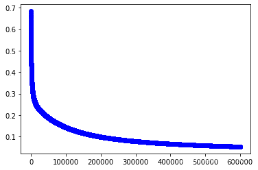
#训练第1个模型
w1,cost_lst1=grandient(data1_x,data1_y,iter_num,alpha)

plt.plot(range(iter_num),cost_lst1,"b-o")

[<matplotlib.lines.Line2D at 0x25624eb08e0>]

#训练第2个模型
w2,cost_lst2=grandient(data2_x,data2_y,iter_num,alpha)
plt.plot(range(iter_num),cost_lst2,"b-o")

[<matplotlib.lines.Line2D at 0x25631b87a60>]

#训练第3个模型
w3,cost_lst3=grandient(data3_x,data3_y,iter_num,alpha)
plt.plot(range(iter_num),cost_lst3,"b-o")

[<matplotlib.lines.Line2D at 0x2562bcdfac0>]

#训练第4个模型
w4,cost_lst4=grandient(data4_x,data4_y,iter_num,alpha)
plt.plot(range(iter_num),cost_lst4,"b-o")

[<matplotlib.lines.Line2D at 0x25631ff4ee0>]

2.5 利用模型进行预测

data_x

array([[ 2.11663151e+00,  7.97280013e+00, -9.32896918e+00,-8.22460526e+00, -1.21784287e+01,  5.49844655e+00],[ 1.88644899e+00,  4.62100554e+00,  2.84159548e+00,4.31244563e-01, -2.47135027e+00,  2.50783257e+00],[ 2.39132949e+00,  6.46460915e+00, -9.80590050e+00,-7.28996786e+00, -9.65098460e+00,  6.38845956e+00],...,[ 2.03146167e+00,  7.80442707e+00, -8.53951210e+00,-9.82440872e+00, -1.00469351e+01,  6.91808489e+00],[ 4.08188906e+00,  6.12768483e+00,  1.10911262e+01,4.81201082e+00, -5.91530191e-03,  5.34221079e+00],[ 9.85744105e-01,  7.28573657e+00, -8.39593964e+00,-6.58647097e+00, -9.65176507e+00,  6.65101187e+00]])

data_x=np.insert(data_x,0,1,axis=1)

data_x.shape

(200, 7)

w3.shape

(7, 1)

multi_pred=pd.DataFrame(zip(h(data_x,w1).ravel(),h(data_x,w2).ravel(),h(data_x,w3).ravel(),h(data_x,w4).ravel()))
multi_pred

	0	1	2	3
0	0.020436	4.556248e-15	9.999975e-01	2.601227e-27
1	0.820488	4.180906e-05	3.551499e-05	5.908691e-05
2	0.109309	7.316201e-14	9.999978e-01	7.091713e-24
3	0.036608	9.999562e-01	1.048562e-09	5.724854e-03
4	0.003075	9.999292e-01	2.516742e-09	6.423038e-05
...	...	...	...	...
195	0.017278	3.221293e-06	3.753372e-14	9.999943e-01
196	0.003369	9.999966e-01	6.673394e-10	2.281428e-03
197	0.000606	1.118174e-13	9.999941e-01	1.780212e-28
198	0.013072	4.999118e-05	9.811154e-14	9.996689e-01
199	0.151548	1.329623e-13	9.999447e-01	2.571989e-24

200 rows × 4 columns

2.6 计算准确率

np.sum(np.argmax(multi_pred.values,axis=1)==data_y.ravel())/len(data)

1.0

查看全文

http://www.lryc.cn/news/104053.html

【ChatGLM_01】ChatGLM2-6B本地安装与部署（大语言模型）

谷歌Tsunami(海啸)扫描器搭建扩展使用教程

诚迈科技承办大同首届信息技术产业峰会，共话数字经济崭新未来

【Python】Python使用TK实现动态爱心效果

Unity3d C#快速打开萤石云监控视频流（ezopen）支持WebGL平台，替代UMP播放视频流的方案（含源码）

【Android】APP启动优化学习笔记

docker的使用

iOS使用Rust调研

抖音引流推广的几个方法，抖音全自动引流脚本软件详细使用教学

k8s概念-DaemonSet

Mac 终端快捷键设置：如何给 Mac 中的 Terminal 设置 Ctrl+Alt+T 快捷键快速启动

VR 变电站事故追忆反演——正泰电力携手图扑

fpga开发——蜂鸣器

【Liux下6818开发板(ARM)】触摸屏

苍穹外卖day11——数据统计图形报表（Apache ECharts）

在制作PC端Game Launcher游戏启动器时涉及到的技术选型

SQL力扣练习（九）

软考高级架构师笔记-10数学计算题

设计模式五：建造者模式(Builder Pattern)

C++多线程编程(包含c++20内容)

【C语言】通讯录2.0 （动态增长版）

详解AMQP协议以及JAVA体系中的AMQP

跨境电商外贸常态下，深度分析Live Market的优势

vue2企业级项目（八）

小研究 - 主动式微服务细粒度弹性缩放算法研究（二）

【雕爷学编程】Arduino动手做（177）---ESP-32 掌控板

使用Gunicorn+Nginx部署Flask项目

【12】STM32·HAL库开发-STM32时钟系统 | F1/F4/F7时钟树 | 配置系统时钟

Kotlin基础（十）：函数进阶

计算机视觉（四）神经网络与典型的机器学习步骤

	F1	F2	F3	F4	target
0	5.1	3.5	1.4	0.2	0.0
1	4.9	3.0	1.4	0.2	0.0
2	4.7	3.2	1.3	0.2	0.0
3	4.6	3.1	1.5	0.2	0.0
4	5.0	3.6	1.4	0.2	0.0
...	...	...	...	...	...
145	6.7	3.0	5.2	2.3	2.0
146	6.3	2.5	5.0	1.9	2.0
147	6.5	3.0	5.2	2.0	2.0
148	6.2	3.4	5.4	2.3	2.0
149	5.9	3.0	5.1	1.8	2.0

	ones	F1	F2	F3	F4	target
0	1	5.1	3.5	1.4	0.2	0.0
1	1	4.9	3.0	1.4	0.2	0.0
2	1	4.7	3.2	1.3	0.2	0.0
3	1	4.6	3.1	1.5	0.2	0.0
4	1	5.0	3.6	1.4	0.2	0.0
...	...	...	...	...	...	...
145	1	6.7	3.0	5.2	2.3	2.0
146	1	6.3	2.5	5.0	1.9	2.0
147	1	6.5	3.0	5.2	2.0	2.0
148	1	6.2	3.4	5.4	2.3	2.0
149	1	5.9	3.0	5.1	1.8	2.0

	ones	F1	F2	F3	F4	target
0	1	5.1	3.5	1.4	0.2	0
1	1	4.9	3.0	1.4	0.2	0
2	1	4.7	3.2	1.3	0.2	0
3	1	4.6	3.1	1.5	0.2	0
4	1	5.0	3.6	1.4	0.2	0
...	...	...	...	...	...	...
145	1	6.7	3.0	5.2	2.3	2
146	1	6.3	2.5	5.0	1.9	2
147	1	6.5	3.0	5.2	2.0	2
148	1	6.2	3.4	5.4	2.3	2
149	1	5.9	3.0	5.1	1.8	2

	ones	F1	F2	F3	F4	target
0	1	5.1	3.5	1.4	0.2	0
1	1	4.9	3.0	1.4	0.2	0
2	1	4.7	3.2	1.3	0.2	0
3	1	4.6	3.1	1.5	0.2	0
4	1	5.0	3.6	1.4	0.2	0
...	...	...	...	...	...	...
145	1	6.7	3.0	5.2	2.3	2
146	1	6.3	2.5	5.0	1.9	2
147	1	6.5	3.0	5.2	2.0	2
148	1	6.2	3.4	5.4	2.3	2
149	1	5.9	3.0	5.1	1.8	2

	ones	F1	F2	F3	F4	target
0	1	5.1	3.5	1.4	0.2	1
1	1	4.9	3.0	1.4	0.2	1
2	1	4.7	3.2	1.3	0.2	1
3	1	4.6	3.1	1.5	0.2	1
4	1	5.0	3.6	1.4	0.2	1
...	...	...	...	...	...	...
145	1	6.7	3.0	5.2	2.3	0
146	1	6.3	2.5	5.0	1.9	0
147	1	6.5	3.0	5.2	2.0	0
148	1	6.2	3.4	5.4	2.3	0
149	1	5.9	3.0	5.1	1.8	0

	ones	F1	F2	F3	F4	target
50	1	7.0	3.2	4.7	1.4	1
51	1	6.4	3.2	4.5	1.5	1
52	1	6.9	3.1	4.9	1.5	1
53	1	5.5	2.3	4.0	1.3	1
54	1	6.5	2.8	4.6	1.5	1

	ones	F1	F2	F3	F4	target
0	1	5.1	3.5	1.4	0.2	0
1	1	4.9	3.0	1.4	0.2	0
2	1	4.7	3.2	1.3	0.2	0
3	1	4.6	3.1	1.5	0.2	0
4	1	5.0	3.6	1.4	0.2	0
...	...	...	...	...	...	...
145	1	6.7	3.0	5.2	2.3	1
146	1	6.3	2.5	5.0	1.9	1
147	1	6.5	3.0	5.2	2.0	1
148	1	6.2	3.4	5.4	2.3	1
149	1	5.9	3.0	5.1	1.8	1

	模型1	模糊2	模型3
0	1	0	0
1	1	0	0
2	1	0	0
3	1	0	0
4	1	0	0
...	...	...	...
145	0	0	1
146	0	1	1
147	0	0	1
148	0	0	1
149	0	0	1

	F1	F2	F3	F4	target
0	5.1	3.5	1.4	0.2	0.0
1	4.9	3.0	1.4	0.2	0.0
2	4.7	3.2	1.3	0.2	0.0
3	4.6	3.1	1.5	0.2	0.0
4	5.0	3.6	1.4	0.2	0.0
...	...	...	...	...	...
145	6.7	3.0	5.2	2.3	2.0
146	6.3	2.5	5.0	1.9	2.0
147	6.5	3.0	5.2	2.0	2.0
148	6.2	3.4	5.4	2.3	2.0
149	5.9	3.0	5.1	1.8	2.0

	ones	F1	F2	F3	F4	target
0	1	5.1	3.5	1.4	0.2	0.0
1	1	4.9	3.0	1.4	0.2	0.0
2	1	4.7	3.2	1.3	0.2	0.0
3	1	4.6	3.1	1.5	0.2	0.0
4	1	5.0	3.6	1.4	0.2	0.0
...	...	...	...	...	...	...
145	1	6.7	3.0	5.2	2.3	2.0
146	1	6.3	2.5	5.0	1.9	2.0
147	1	6.5	3.0	5.2	2.0	2.0
148	1	6.2	3.4	5.4	2.3	2.0
149	1	5.9	3.0	5.1	1.8	2.0

	ones	F1	F2	F3	F4	target
0	1	5.1	3.5	1.4	0.2	0
1	1	4.9	3.0	1.4	0.2	0
2	1	4.7	3.2	1.3	0.2	0
3	1	4.6	3.1	1.5	0.2	0
4	1	5.0	3.6	1.4	0.2	0
...	...	...	...	...	...	...
145	1	6.7	3.0	5.2	2.3	2
146	1	6.3	2.5	5.0	1.9	2
147	1	6.5	3.0	5.2	2.0	2
148	1	6.2	3.4	5.4	2.3	2
149	1	5.9	3.0	5.1	1.8	2

	ones	F1	F2	F3	F4	target
0	1	5.1	3.5	1.4	0.2	0
1	1	4.9	3.0	1.4	0.2	0
2	1	4.7	3.2	1.3	0.2	0
3	1	4.6	3.1	1.5	0.2	0
4	1	5.0	3.6	1.4	0.2	0
...	...	...	...	...	...	...
145	1	6.7	3.0	5.2	2.3	2
146	1	6.3	2.5	5.0	1.9	2
147	1	6.5	3.0	5.2	2.0	2
148	1	6.2	3.4	5.4	2.3	2
149	1	5.9	3.0	5.1	1.8	2

	ones	F1	F2	F3	F4	target
0	1	5.1	3.5	1.4	0.2	1
1	1	4.9	3.0	1.4	0.2	1
2	1	4.7	3.2	1.3	0.2	1
3	1	4.6	3.1	1.5	0.2	1
4	1	5.0	3.6	1.4	0.2	1
...	...	...	...	...	...	...
145	1	6.7	3.0	5.2	2.3	0
146	1	6.3	2.5	5.0	1.9	0
147	1	6.5	3.0	5.2	2.0	0
148	1	6.2	3.4	5.4	2.3	0
149	1	5.9	3.0	5.1	1.8	0

	ones	F1	F2	F3	F4	target
50	1	7.0	3.2	4.7	1.4	1
51	1	6.4	3.2	4.5	1.5	1
52	1	6.9	3.1	4.9	1.5	1
53	1	5.5	2.3	4.0	1.3	1
54	1	6.5	2.8	4.6	1.5	1

	ones	F1	F2	F3	F4	target
0	1	5.1	3.5	1.4	0.2	0
1	1	4.9	3.0	1.4	0.2	0
2	1	4.7	3.2	1.3	0.2	0
3	1	4.6	3.1	1.5	0.2	0
4	1	5.0	3.6	1.4	0.2	0
...	...	...	...	...	...	...
145	1	6.7	3.0	5.2	2.3	1
146	1	6.3	2.5	5.0	1.9	1
147	1	6.5	3.0	5.2	2.0	1
148	1	6.2	3.4	5.4	2.3	1
149	1	5.9	3.0	5.1	1.8	1

	模型1	模糊2	模型3
0	1	0	0
1	1	0	0
2	1	0	0
3	1	0	0
4	1	0	0
...	...	...	...
145	0	0	1
146	0	1	1
147	0	0	1
148	0	0	1
149	0	0	1

文章目录

多分类以及机器学习实践

如何对多个类别进行分类

1.1 数据的预处理

1.2 训练数据的准备

1.3 定义假设函数，代价函数，梯度下降算法（从实验3复制过来）

1.4 调用梯度下降算法来学习三个分类模型的参数

1.5 利用模型进行预测

1.6 评估模型

1.7 试试sklearn

实验4(1) 请动手完成你们第一个多分类问题，祝好运！完成下面代码

2.1 数据读取

2.2 训练数据的准备

2.3 定义假设函数、代价函数和梯度下降算法

2.4 学习这四个分类模型

2.5 利用模型进行预测

2.6 计算准确率

相关文章：

	F1	F2	F3	F4	target
0	5.1	3.5	1.4	0.2	0.0
1	4.9	3.0	1.4	0.2	0.0
2	4.7	3.2	1.3	0.2	0.0
3	4.6	3.1	1.5	0.2	0.0
4	5.0	3.6	1.4	0.2	0.0
...	...	...	...	...	...
145	6.7	3.0	5.2	2.3	2.0
146	6.3	2.5	5.0	1.9	2.0
147	6.5	3.0	5.2	2.0	2.0
148	6.2	3.4	5.4	2.3	2.0
149	5.9	3.0	5.1	1.8	2.0

	ones	F1	F2	F3	F4	target
0	1	5.1	3.5	1.4	0.2	0.0
1	1	4.9	3.0	1.4	0.2	0.0
2	1	4.7	3.2	1.3	0.2	0.0
3	1	4.6	3.1	1.5	0.2	0.0
4	1	5.0	3.6	1.4	0.2	0.0
...	...	...	...	...	...	...
145	1	6.7	3.0	5.2	2.3	2.0
146	1	6.3	2.5	5.0	1.9	2.0
147	1	6.5	3.0	5.2	2.0	2.0
148	1	6.2	3.4	5.4	2.3	2.0
149	1	5.9	3.0	5.1	1.8	2.0

	ones	F1	F2	F3	F4	target
0	1	5.1	3.5	1.4	0.2	0
1	1	4.9	3.0	1.4	0.2	0
2	1	4.7	3.2	1.3	0.2	0
3	1	4.6	3.1	1.5	0.2	0
4	1	5.0	3.6	1.4	0.2	0
...	...	...	...	...	...	...
145	1	6.7	3.0	5.2	2.3	2
146	1	6.3	2.5	5.0	1.9	2
147	1	6.5	3.0	5.2	2.0	2
148	1	6.2	3.4	5.4	2.3	2
149	1	5.9	3.0	5.1	1.8	2

	ones	F1	F2	F3	F4	target
0	1	5.1	3.5	1.4	0.2	0
1	1	4.9	3.0	1.4	0.2	0
2	1	4.7	3.2	1.3	0.2	0
3	1	4.6	3.1	1.5	0.2	0
4	1	5.0	3.6	1.4	0.2	0
...	...	...	...	...	...	...
145	1	6.7	3.0	5.2	2.3	2
146	1	6.3	2.5	5.0	1.9	2
147	1	6.5	3.0	5.2	2.0	2
148	1	6.2	3.4	5.4	2.3	2
149	1	5.9	3.0	5.1	1.8	2

	ones	F1	F2	F3	F4	target
0	1	5.1	3.5	1.4	0.2	1
1	1	4.9	3.0	1.4	0.2	1
2	1	4.7	3.2	1.3	0.2	1
3	1	4.6	3.1	1.5	0.2	1
4	1	5.0	3.6	1.4	0.2	1
...	...	...	...	...	...	...
145	1	6.7	3.0	5.2	2.3	0
146	1	6.3	2.5	5.0	1.9	0
147	1	6.5	3.0	5.2	2.0	0
148	1	6.2	3.4	5.4	2.3	0
149	1	5.9	3.0	5.1	1.8	0

	ones	F1	F2	F3	F4	target
50	1	7.0	3.2	4.7	1.4	1
51	1	6.4	3.2	4.5	1.5	1
52	1	6.9	3.1	4.9	1.5	1
53	1	5.5	2.3	4.0	1.3	1
54	1	6.5	2.8	4.6	1.5	1

	ones	F1	F2	F3	F4	target
0	1	5.1	3.5	1.4	0.2	0
1	1	4.9	3.0	1.4	0.2	0
2	1	4.7	3.2	1.3	0.2	0
3	1	4.6	3.1	1.5	0.2	0
4	1	5.0	3.6	1.4	0.2	0
...	...	...	...	...	...	...
145	1	6.7	3.0	5.2	2.3	1
146	1	6.3	2.5	5.0	1.9	1
147	1	6.5	3.0	5.2	2.0	1
148	1	6.2	3.4	5.4	2.3	1
149	1	5.9	3.0	5.1	1.8	1

	模型1	模糊2	模型3
0	1	0	0
1	1	0	0
2	1	0	0
3	1	0	0
4	1	0	0
...	...	...	...
145	0	0	1
146	0	1	1
147	0	0	1
148	0	0	1
149	0	0	1