机器学习项目实战-能源利用率 Part-3(特征工程与特征筛选)
博主前期相关的博客可见下:
机器学习项目实战-能源利用率 Part-1(数据清洗)
机器学习项目实战-能源利用率 Part-2(探索性数据分析)
这部分进行的特征工程与特征筛选。
三 特征工程与特征筛选
一般情况下我们分两步走:特征工程与特征筛选:
特征工程: 概括性来说就是尽可能的多在数据中提取特征,各种数值变换,特征组合,分解等各种手段齐上阵。
特征选择: 就是找到最有价值的那些特征作为我们模型的输入,但是之前做了那么多,可能有些是多余的,有些还没被发现,所以这俩阶段都是一个反复在更新的过程。比如我在建模之后拿到了特征重要性,这就为特征选择做了参考,有些不重要的我可以去掉,那些比较重要的,我还可以再想办法让其做更多变换和组合来促进我的模型。所以特征工程并不是一次性就能解决的,需要通过各种结果来反复斟酌。
3.1 特征变换 与 One-hot encode
有点像分析特征之间的相关性
features = data.copy()
numeric_subset = data.select_dtypes('number')
for col in numeric_subset.columns:if col == 'score':nextelse:numeric_subset['log_' + col] = np.log(abs(numeric_subset[col]) + 0.01)categorical_subset = data[['Borough', 'Largest Property Use Type']]
categorical_subset = pd.get_dummies(categorical_subset)features = pd.concat([numeric_subset, categorical_subset], axis = 1)
features.shape
这段代码的目的是为了生成特征矩阵 features,它包含了原始数据 data 的数值特征和分类特征的处理结果。
首先,代码复制了原始数据 data,并将其赋值给 features。
接下来,通过 select_dtypes('number') 选择了 data 中的数值类型的列,并将结果存储在 numeric_subset 中。
然后,使用一个循环遍历 numeric_subset 的列,对每一列进行处理。对于列名为 ‘score’ 的列,直接跳过(使用 next)。对于其他列,将其绝对值加上一个很小的常数(0.01),然后取对数,并将结果存储在 numeric_subset 中以 ‘log_’ 开头的列名中。
接着,从 data 中选择了 ‘Borough’ 和 ‘Largest Property Use Type’ 两列作为分类特征,并使用 pd.get_dummies 进行独热编码(One-Hot Encoding)得到它们的编码结果,并将结果存储在 categorical_subset 中。
最后,使用 pd.concat 将 numeric_subset 和 categorical_subset 按列方向(axis=1)进行拼接,得到最终的特征矩阵 features。
最后一行代码输出了 features 的形状(行数和列数)。

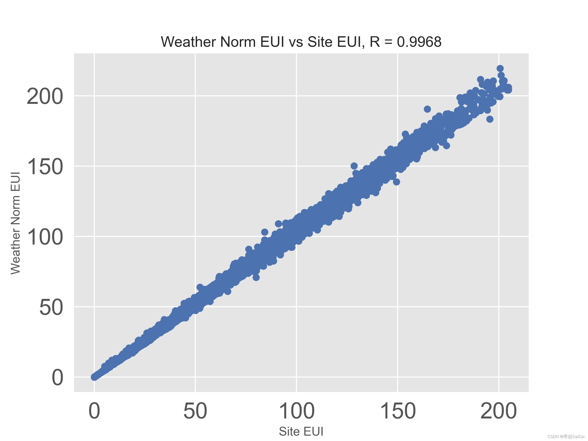
3.2 共线特征
在数据中Site EUI 和 Weather Norm EUI就是要考虑的目标,他俩描述的基本是同一个事
plot_data = data[['Weather Normalized Site EUI (kBtu/ft²)', 'Site EUI (kBtu/ft²)']].dropna()plt.plot(plot_data['Site EUI (kBtu/ft²)'], plot_data['Weather Normalized Site EUI (kBtu/ft²)'], 'bo')
plt.xlabel('Site EUI'); plt.ylabel('Weather Norm EUI')
plt.title('Weather Norm EUI vs Site EUI, R = %.4f' % np.corrcoef(data[['Weather Normalized Site EUI (kBtu/ft²)', 'Site EUI (kBtu/ft²)']].dropna(), rowvar=False)[0][1])
3.3 剔除共线特征
def remove_collinear_features(x, threshold):'''Objective:Remove collinear features in a dataframe with a correlation coefficientgreater than the threshold. Removing collinear features can help a modelto generalize and improves the interpretability of the model.Inputs: threshold: any features with correlations greater than this value are removedOutput: dataframe that contains only the non-highly-collinear features'''y = x['score']x = x.drop(columns = ['score'])corr_matrix = x.corr()iters = range(len(corr_matrix.columns) - 1)drop_cols = []for i in iters:for j in range(i):item = corr_matrix.iloc[j: (j+1), (i+1): (i+2)] col = item.columnsrow = item.indexval = abs(item.values) if val >= threshold:# print(col.values[0], "|", row.values[0], "|", round(val[0][0], 2))drop_cols.append(col.values[0])drops = set(drop_cols)# print(drops)x = x.drop(columns = drops)x = x.drop(columns = ['Weather Normalized Site EUI (kBtu/ft²)', 'Water Use (All Water Sources) (kgal)','log_Water Use (All Water Sources) (kgal)','Largest Property Use Type - Gross Floor Area (ft²)'])x['score'] = yreturn xfeatures = remove_collinear_features(features, 0.6) # 阈值为0.6
features = features.dropna(axis = 1, how = 'all')
print(features.shape)
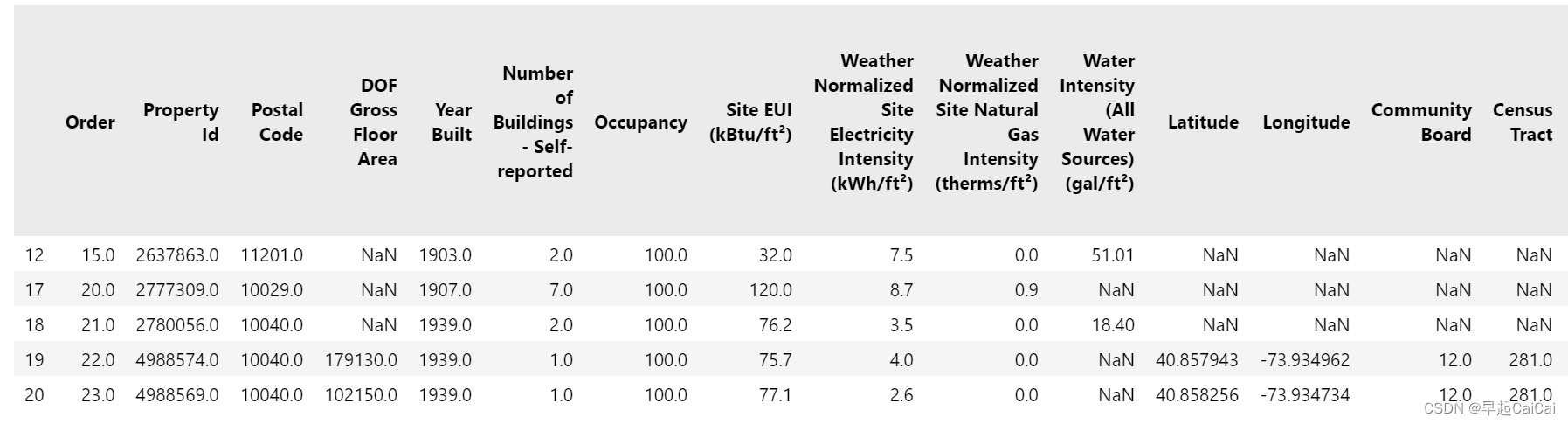
features.head()这段代码定义了一个名为 remove_collinear_features 的函数,用于移除具有高相关性的特征。移除具有高相关性的特征可以帮助模型泛化并提高模型的解释性。
函数的输入参数为 x(包含特征和目标变量的数据框)和 threshold(相关系数的阈值),阈值以上的特征相关性会被移除。
首先,将目标变量 score 存储在变量 y 中,并将其从 x 中移除。
接下来,计算特征之间的相关系数矩阵 corr_matrix。
然后,使用两个嵌套的循环遍历相关系数矩阵中的元素。当相关系数的绝对值大于等于阈值时,将该特征的列名添加到 drop_cols 列表中。
完成循环后,将 drop_cols 转换为集合 drops,以去除重复的特征列名。
然后,从 x 中移除 drops 中的特征列,以及其他预定义的特征列。
接下来,将目标变量 y 添加回 x 中,并将结果返回。
最后,对更新后的特征矩阵 features 进行处理,移除所有包含缺失值的列,并输出其形状(行数和列数),并展示前几行数据。
3.4 数据集划分
no_score = features[features['score'].isna()]
score = features[features['score'].notnull()]
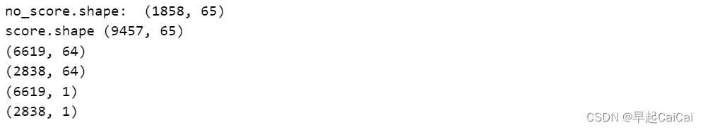
print('no_score.shape: ', no_score.shape)
print('score.shape', score.shape)from sklearn.model_selection import train_test_split
features = score.drop(columns = 'score')
labels = pd.DataFrame(score['score'])
features = features.replace({np.inf: np.nan, -np.inf: np.nan})
X, X_test, y, y_test = train_test_split(features, labels, test_size = 0.3, random_state = 42)
print(X.shape)
print(X_test.shape)
print(y.shape)
print(y_test.shape)
这段代码分为几个步骤:
-
首先,将特征矩阵
features分为两部分:no_score和score。其中,no_score是features中目标变量score为空的部分,而score则是features中目标变量score不为空的部分。 -
输出
no_score和score的形状(行数和列数),分别使用no_score.shape和score.shape打印结果。 -
导入
sklearn.model_selection模块中的train_test_split函数。 -
从
score中移除目标变量score列,得到特征矩阵features。 -
创建标签(目标变量)矩阵
labels,其中只包含目标变量score列。 -
使用
replace方法将features中的无穷大值替换为缺失值(NaN)。 -
使用
train_test_split函数将特征矩阵features和标签矩阵labels划分为训练集和测试集。参数test_size设置测试集的比例为 0.3,random_state设置随机种子为 42。将划分后的结果分别存储在X、X_test、y和y_test中。 -
输出训练集
X、测试集X_test、训练集标签y和测试集标签y_test的形状(行数和列数),分别使用X.shape、X_test.shape、y.shape和y_test.shape打印结果。
这段代码的目的是将数据集划分为训练集和测试集,并准备好用于训练和评估模型的特征矩阵和标签矩阵。
3.5 建立一个Baseline
在建模之前,我们得有一个最坏的打算,就是模型起码得有点作用才行。
# 衡量标准: Mean Absolute Error
def mae(y_true, y_pred):return np.mean(abs(y_true - y_pred))baseline_guess = np.median(y)print('The baseline guess is a score of %.2f' % baseline_guess)
print('Baseline Performance on the test set: MAE = %.4f' % mae(y_test, baseline_guess))
这段代码定义了一个衡量标准函数 mae,并计算了一个基准预测结果。
-
mae函数计算了预测值与真实值之间的平均绝对误差(Mean Absolute Error)。它接受两个参数y_true和y_pred,分别表示真实值和预测值。函数内部通过np.mean(abs(y_true - y_pred))计算平均绝对误差,并返回结果。 -
baseline_guess是基准预测的结果,它被设置为标签(目标变量)y的中位数。这相当于一种简单的基准方法,用中位数作为所有预测的固定值。 -
使用
print函数打印基准预测结果的信息。'The baseline guess is a score of %.2f' % baseline_guess会输出基准预测结果的值,保留两位小数。'Baseline Performance on the test set: MAE = %.4f' % mae(y_test, baseline_guess)会输出基准预测结果在测试集上的性能,即平均绝对误差(MAE),保留四位小数。
这段代码的目的是计算基准预测结果,并输出基准预测结果的信息以及在测试集上的性能评估(使用平均绝对误差作为衡量标准)。

3.6 保存数据
no_score.to_csv('data/no_score.csv', index = False)
X.to_csv('data/training_features.csv', index = False)
X_test.to_csv('data/testing_features.csv', index = False)
y.to_csv('data/training_labels.csv', index = False)
y_test.to_csv('data/testing_labels.csv', index = False)
Reference
机器学习项目实战-能源利用率 Part-1(数据清洗)
机器学习项目实战-能源利用率 Part-2(探索性数据分析)
机器学习项目实战-能源利用率1-数据预处理