台北房价预测
目录
- 1.数据理解
- 1.1分析数据集的基本结构,查询并输出数据的前 10 行和 后 10 行
- 1.2识别并输出所有变量
- 2.数据清洗
- 2.1输出所有变量折线图
- 2.2缺失值处理
- 2.3异常值处理
- 3.数据分析
- 3.1寻找相关性
- 3.2划分数据集
- 4.数据整理
- 4.1数据标准化
- 5.回归预测分析
- 5.1线性回归&岭回归&套索回归
- 6.可视化
- 6.1均分方差
- 6.2平均绝对误差
- 6.3 所有预测值与真实值对比
1.数据理解
from sklearn import model_selection as ms
from sklearn.preprocessing import StandardScaler
from sklearn import linear_model
from sklearn.metrics import accuracy_score
from sklearn.preprocessing import PolynomialFeatures as Poly
from sklearn.metrics import mean_squared_error, mean_absolute_error, r2_score
import pandas as pd
import numpy as np
import matplotlib.pyplot as pltdata=pd.read_excel("台北房产数据集.xlsx")
1.1分析数据集的基本结构,查询并输出数据的前 10 行和 后 10 行
#前十行
data.head(10)

#后十行
data.tail(10)
1.2识别并输出所有变量
data.dtypes

2.数据清洗
2.1输出所有变量折线图
便于观察观察所有特征的数据。
from pylab import mpl
# 设置显示中文字体
mpl.rcParams["font.sans-serif"] = ["SimHei"]
# 绘制直方图
data.hist(bins=50, figsize=(20,15))


2.2缺失值处理
查看每一列的缺失值
#查看每一列的缺失值
data.isnull().sum()

由于缺失值较少,删除具有缺失值的行不会对数据有太大改变。
#删除具有空值的行
data=data.dropna()
data.shape
#(412, 8)
2.3异常值处理
在上面的直方图中我们可以看到有部分数值是与之前的数值格格不入的;
比如附近便利店的数量达到70多个、单位房价值异常高;
我们把这些异常值的行取平均数填入;
- 先找到数量异常的行
- 再计算该列的平均值
- 最后将该行个数替换为列的平均
#在上面的直方图中我们可以看到有部分数值是与之前的数值格格不入的
#比如附近便利店的数量达到70多个、单位房价值异常高
#我们把这些异常值的行取平均数填入#先找到便利店数量异常的行
data.loc[data['X4 附近便利店家数']>50]
print("异常行的数量:",data.loc[data['X4 附近便利店家数']>50].shape[0])

#将该行便利店个数替换为列的平均值#先计算该列的平均值
shop_avg=(int)(data['X4 附近便利店家数'].mean())
print("附近便利店家数的平均值为:",shop_avg)
data["X4 附近便利店家数"]=data["X4 附近便利店家数"].replace({70:shop_avg})
print("异常行的数量:",data.loc[data['X4 附近便利店家数']>50].shape[0])

#先找到单位面积房价异常的行
data.loc[data['Y 单位面积房价']>100]
# print("异常行的数量:",data.loc[data['Y 单位面积房价']>100].shape[0])

#将该行单位房价替换为列的平均值#先计算该列的平均值
shop_avg=(int)(data['Y 单位面积房价'].mean())
print("单位面积房价的平均值为:",shop_avg)
data["Y 单位面积房价"]=data["Y 单位面积房价"].replace({117.5:shop_avg})
print("异常行的数量:",data.loc[data['Y 单位面积房价']>100].shape[0])

3.数据分析
3.1寻找相关性
由于有些特征可能对房价起不到太大作用,还有可能与目标标签是负相关的关系,放到训练集里面既是浪费算力也会减少模型的准确性。
我们数据分析的第一步就是寻找相关性,相关系数范围 [-1, 1] ,越接近 1 表示有越强的正相关,越接近 -1 表示有越强的负相关:
#寻找相关性,相关系数范围 [-1, 1] ,越接近 1 表示有越强的正相关,越接近 -1 表示有越强的负相关
corr_matrix = data.corr()
corr_matrix

#具体看每个属性与单位面积房价的相关性
corr_matrix["Y 单位面积房价"].sort_values(ascending=False)

由上面相关性可知便利店家数与经纬度的相关性较高,而交易年月虽是正相关,但趋近于零,而负相关的变量我们就不考虑了。
#定义散点图函数
def scatter_figure(th1,th2):data.plot(kind="scatter", x=th1, y=th2)plt.xlabel(th1)plt.ylabel(th2)data.plot(kind="scatter", x=th1, y=th2, alpha=0.3)plt.xlabel(th1)plt.ylabel(th2)
# 经度和单位房价的散点图与高密度点
scatter_figure('X6 经度','Y 单位面积房价')

# 纬度和单位房价的散点图与高密度点
scatter_figure('X5 纬度','Y 单位面积房价')

# 经度和纬度的散点图,查看在哪个区域的房价高低,与高密度点
scatter_figure('X6 经度','X5 纬度')

3.2划分数据集
我们把数据集按照训练集:测试集为7:3进行划分。
而特征值采用附近便利店数与经纬度这三列数据。
#划分数据集
y=data[['Y 单位面积房价']]
x=data[['X4 附近便利店家数','X5 纬度','X6 经度']]
x_train, x_test, y_train, y_test = ms.train_test_split(x, y, random_state=1, test_size=0.3)
x_train.head()

4.数据整理
4.1数据标准化
#标准化
std = StandardScaler()
x_train_std = std.fit_transform(x_train)
x_test_std = std.fit_transform(x_test)
print("标准化之前:\n",x_test)
print("标准化之后:\n",x_test_std)
标准化之前:

标准化之后:

5.回归预测分析
5.1线性回归&岭回归&套索回归
回归预测这一部分我们采用了三种回归模型来训练与预测。
三种模型得分:
#初始化训练器
line = linear_model.LinearRegression()
ridge=linear_model.Ridge()
lasso=linear_model.Lasso()nums=[1,2,3]
for num in nums:#用于生成多项式特征,即将输入数据的特征进行组合,生成新的特征poly= Poly(num) x_train_poly= poly.fit_transform(x_train_std)x_test_poly= poly.transform(x_test_std)line.fit(x_train_poly,y_train)ridge.fit(x_train_poly,y_train)lasso.fit(x_train_poly,y_train)# print("预测值为:",y_pred)# print("模型预测的均方误差:",mean_squared_error(y_test,y_test_pred))print("第{}轮训练结果:".format(num))print("线性回归模型得分:",line.score(x_test_poly,y_test))print("岭回归模型得分:",ridge.score(x_test_poly,y_test))print("套索回归模型得分:",lasso.score(x_test_poly,y_test))print("------------------------------------------------------")#预测
y_test_line_pred=line.predict(x_test_poly)
y_test_ridge_pred=ridge.predict(x_test_poly)
y_test_lasso_pred=lasso.predict(x_test_poly)

从得分中我们可以看出来线性回归与岭回归模型得分几乎相等,而套索回归模型稍逊色些。
部分预测值与实际值对比:
x=[]
for a in range(60):x.append([a+20])
# print(x)
y_test2=y_test[20:80]
y_line_pred=y_test_line_pred[20:80]
y_ridge_pred=y_test_ridge_pred[20:80]
y_lasso_pred=y_test_lasso_pred[20:80]
#设置图形
plt.figure(figsize=(20,8),dpi=80)
#画图,zoder是控制画图流程的属性,其值越大则表示画图的时间越晚
plt.plot(x,y_test2,color='tomato',linestyle='--',label='准确值',marker='o')
plt.plot(x,y_line_pred,color='orange',label='线性回归预测值')
plt.plot(x,y_ridge_pred,color='deepskyblue',label='岭回归回归预测值')
plt.plot(x,y_lasso_pred,color='seagreen',label='套索回归预测值')plt.xlabel("个数")#给x轴起名字
plt.ylabel("对比")#给y轴起名字
plt.grid()  # 设置网格模式
plt.title("部分预测值与实际值对比图")
plt.legend()
#设置每个点上的数值
#展示
plt.show()
6.可视化
# 计算均分方差
train_MSE_line = [mean_squared_error(y_test, [np.mean(y_test)] * len(y_test)),mean_squared_error(y_test, y_test_line_pred)]
train_MSE_ridge = [mean_squared_error(y_test, [np.mean(y_test)] * len(y_test)),mean_squared_error(y_test, y_test_ridge_pred)]
train_MSE_lasso = [mean_squared_error(y_test, [np.mean(y_test)] * len(y_test)),mean_squared_error(y_test, y_test_lasso_pred)]#计算平均绝对误差
train_MAE_line = [mean_absolute_error(y_test, [np.mean(y_test)] * len(y_test)),mean_absolute_error(y_test, y_test_line_pred)]
train_MAE_ridge = [mean_absolute_error(y_test, [np.mean(y_test)] * len(y_test)),mean_absolute_error(y_test, y_test_ridge_pred)]
train_MAE_lasso = [mean_absolute_error(y_test, [np.mean(y_test)] * len(y_test)),mean_absolute_error(y_test, y_test_lasso_pred)]# 绘图函数
def figure(title, *datalist):print(datalist)plt.figure(facecolor='gray', figsize=[16, 8])for v in datalist:plt.plot(v[0], '-', label=v[1], linewidth=2)plt.plot(v[0], 'o')plt.grid()plt.title(title, fontsize=20)plt.legend(fontsize=16)plt.show()
6.1均分方差
# 绘制误差图
#figure(' 均分方差 = %.4f' % (train_MSE_line[-1]), [train_MSE_line, 'MSE'])
figure('line均分方差=%.4f   ridge均分方差=%.4f   lasso均分方差=%.4f' % (train_MSE_line[-1],train_MSE_ridge[-1],train_MSE_lasso[-1]),[train_MSE_line, '线性回归MSE'],[train_MSE_ridge, '岭回归MSE'],[train_MSE_lasso, '套索MSE'])

6.2平均绝对误差
figure('line平均绝对误差=%.4f ridge平均绝对误差=%.4f lasso平均绝对误差=%.4f' % (train_MAE_line[-1],train_MAE_ridge[-1],train_MAE_lasso[-1]),[train_MAE_line, '线性回归MAE'],[train_MAE_ridge, '岭回归MAE'],[train_MAE_lasso, '套索MAE'])

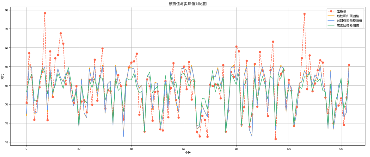
6.3 所有预测值与真实值对比
x=[]
for a in range(124):x.append([a])
#设置图形
plt.figure(figsize=(20,8),dpi=80)
#画图,zoder是控制画图流程的属性,其值越大则表示画图的时间越晚
plt.plot(x,y_test,color='tomato',linestyle='--',label='准确值',marker='o')
plt.plot(x,y_test_line_pred,color='orange',label='线性回归预测值')
plt.plot(x,y_test_ridge_pred,color='cornflowerblue',label='岭回归回归预测值')
plt.plot(x,y_test_lasso_pred,color='mediumseagreen',label='套索回归预测值')plt.xlabel("个数")#给x轴起名字
plt.ylabel("对比")#给y轴起名字
plt.grid()  # 设置网格模式
plt.title("预测值与实际值对比图")
plt.legend()
#设置每个点上的数值
#展示
plt.show()