基于CNN图像特征提取流程（简化版）

前言

心血来潮想把下面的又矩阵换成图片看一下，但是图像像素点太多了，处理效果不是很明显，后面用其他的卷积核弄了一下。

卷积神经网络(CNN)处理流程（简化版）-CSDN博客https://blog.csdn.net/weixin_64066303/article/details/149662869?spm=1001.2014.3001.5501

特征提取 

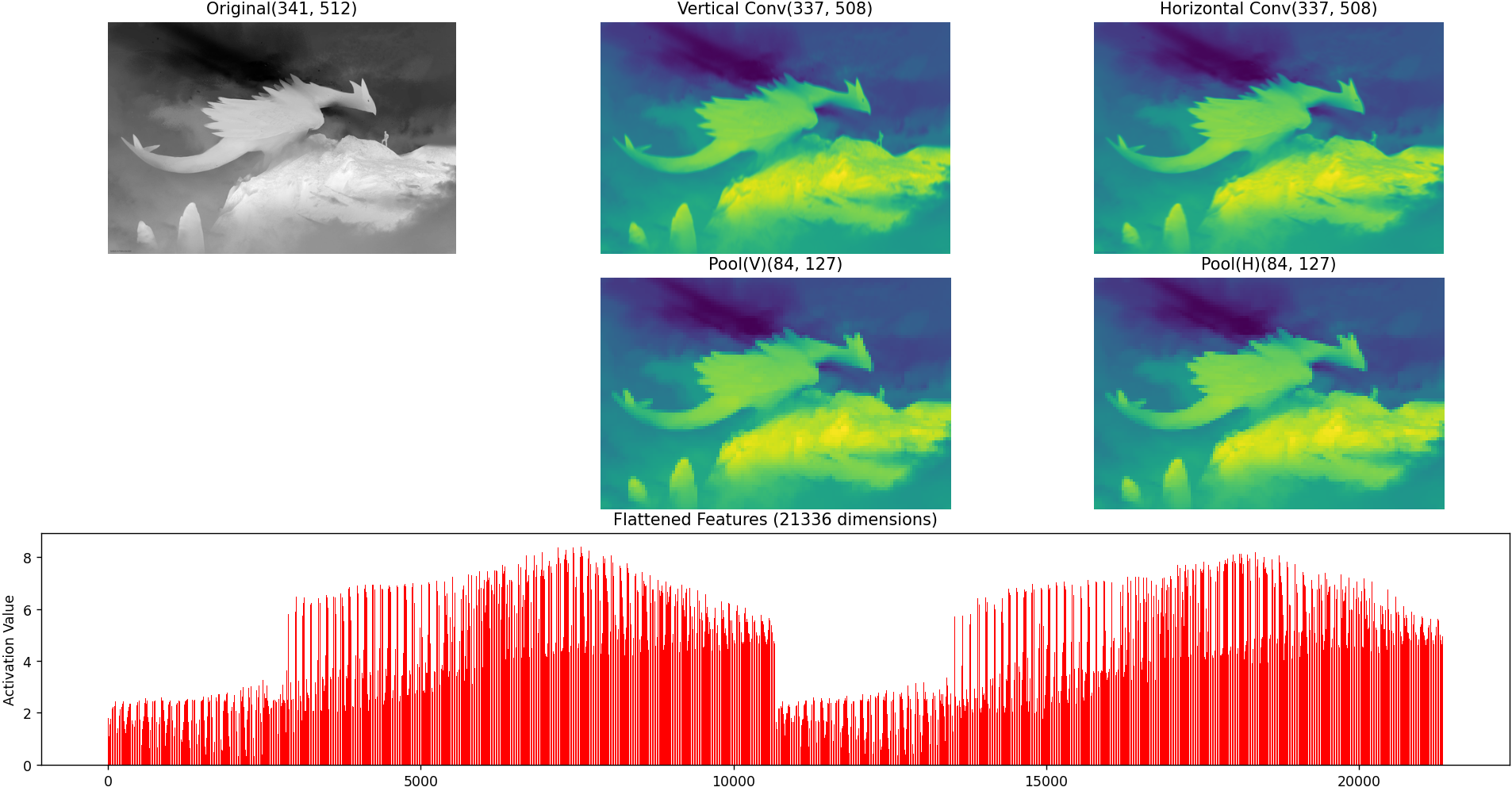
代码实现了一个基于卷积神经网络（CNN）的图像特征提取流程，首先加载并预处理灰度图像（调整大小、归一化和反色），然后分别使用5×5的垂直和水平边缘检测卷积核进行特征提取，接着通过ReLU激活函数引入非线性并去除负值，再经过4×4的最大池化降低特征图维度，最后将两个方向的池化特征展平拼接成一维向量。整个过程模拟了CNN的特征提取过程，并通过可视化展示了各阶段（原始图像、卷积结果、池化特征和扁平化向量）的处理效果，有助于理解图像在CNN中的特征变换过程。

# 定义更大的卷积核（5x5）kernel_v = np.array([[0, 0.5, 1, 0.5, 0],[0, 0.5, 1, 0.5, 0],[0, 0.5, 1, 0.5, 0],[0, 0.5, 1, 0.5, 0],[0, 0.5, 1, 0.5, 0]])  # 垂直边缘检测kernel_h = np.array([[0, 0, 0, 0, 0],[0.5, 0.5, 0.5, 0.5, 0.5],[1, 1, 1, 1, 1],[0.5, 0.5, 0.5, 0.5, 0.5],[0, 0, 0, 0, 0]])  # 水平边缘检测

import numpy as np
import matplotlib.pyplot as plt
from PIL import Image
from skimage.util import view_as_blocks
import timedef load_and_resize_image(image_path, max_size=512):  # 增大默认尺寸以保留更多细节"""加载图片并等比例缩小"""print("⏳ 正在加载图片...")start_time = time.time()img = Image.open(image_path).convert('L')original_size = img.size# 等比例缩小ratio = min(max_size / original_size[0], max_size / original_size[1])new_size = (int(original_size[0] * ratio), int(original_size[1] * ratio))img = img.resize(new_size, Image.LANCZOS)img_array = np.array(img)img_array = img_array / 255.0  # 归一化img_array = 1 - img_array  # 反色print(f"✅ 图片加载完成 | 原始尺寸: {original_size} | 处理后尺寸: {new_size} | 耗时: {time.time() - start_time:.2f}s")return img_arraydef conv2d(image, kernel, operation_name=""):"""带进度提示的2D卷积"""print(f"⏳ 正在计算{operation_name}卷积...")start_time = time.time()h, w = image.shapek_h, k_w = kernel.shapeoutput = np.zeros((h - k_h + 1, w - k_w + 1))total_steps = h - k_h + 1for y in range(h - k_h + 1):if y % 10 == 0 or y == total_steps - 1:print(f"  进度: {y + 1}/{total_steps}行", end='\r')for x in range(w - k_w + 1):output[y, x] = np.sum(image[y:y + k_h, x:x + k_w] * kernel)print(f"✅ {operation_name}卷积完成 | 耗时: {time.time() - start_time:.2f}s")return outputdef maxpool2d(image, pool_size=4):  # 增大默认池化尺寸"""最大池化"""print(f"⏳ 正在进行{pool_size}x{pool_size}最大池化...")start_time = time.time()h, w = image.shapeh = h - h % pool_sizew = w - w % pool_sizeimage = image[:h, :w]blocks = view_as_blocks(image, (pool_size, pool_size))pooled = blocks.max(axis=2).max(axis=2)print(f"✅ 池化完成 | 耗时: {time.time() - start_time:.2f}s")return pooleddef visualize_full_process(original, conv_v, conv_h, relu_v, relu_h, pool_v, pool_h, flattened):"""完整可视化处理流程"""plt.figure(figsize=(18, 12))  # 增大画布尺寸# 原始图像plt.subplot(3, 3, 1)plt.imshow(original, cmap='gray')plt.title(f'Original{original.shape}')plt.axis('off')# 垂直卷积plt.subplot(3, 3, 2)plt.imshow(conv_v, cmap='viridis')plt.title(f'Vertical Conv{conv_v.shape}')plt.axis('off')# 水平卷积plt.subplot(3, 3, 3)plt.imshow(conv_h, cmap='viridis')plt.title(f'Horizontal Conv{conv_h.shape}')plt.axis('off')# 池化垂直plt.subplot(3, 3, 5)plt.imshow(pool_v, cmap='viridis')plt.title(f'Pool(V){pool_v.shape}')plt.axis('off')# 池化水平plt.subplot(3, 3, 6)plt.imshow(pool_h, cmap='viridis')plt.title(f'Pool(H){pool_h.shape}')plt.axis('off')# 扁平化特征plt.subplot(3, 1, 3)plt.bar(range(len(flattened)), flattened, color=['red' if x > 0 else 'blue' for x in flattened])plt.title(f'Flattened Features ({len(flattened)} dimensions)')plt.xlabel('Feature Index')plt.ylabel('Activation Value')plt.tight_layout()plt.show()def process_image(image_path, max_size=512, pool_size=4):  # 增大默认参数"""完整的图像处理流程"""print("\n" + "=" * 50)print("🚀 开始图像处理流程")print("=" * 50)# 1. 加载和预处理original = load_and_resize_image(image_path, max_size)# 定义更大的卷积核（5x5）kernel_v = np.array([[0, 0.5, 1, 0.5, 0],[0, 0.5, 1, 0.5, 0],[0, 0.5, 1, 0.5, 0],[0, 0.5, 1, 0.5, 0],[0, 0.5, 1, 0.5, 0]])  # 垂直边缘检测kernel_h = np.array([[0, 0, 0, 0, 0],[0.5, 0.5, 0.5, 0.5, 0.5],[1, 1, 1, 1, 1],[0.5, 0.5, 0.5, 0.5, 0.5],[0, 0, 0, 0, 0]])  # 水平边缘检测# 2. 卷积conv_v = conv2d(original, kernel_v, "垂直")conv_h = conv2d(original, kernel_h, "水平")# 3. ReLU激活print("⏳ 应用ReLU激活函数...")relu_v = np.maximum(0, conv_v)relu_h = np.maximum(0, conv_h)print("✅ ReLU激活完成")# 4. 池化pool_v = maxpool2d(relu_v, pool_size)pool_h = maxpool2d(relu_h, pool_size)# 5. 扁平化print("⏳ 正在扁平化特征...")flattened = np.concatenate([pool_v.flatten(), pool_h.flatten()])print(f"✅ 扁平化完成 | 特征维度: {len(flattened)}")# 可视化visualize_full_process(original, conv_v, conv_h, relu_v, relu_h, pool_v, pool_h, flattened)return {'original': original,'conv_v': conv_v,'conv_h': conv_h,'relu_v': relu_v,'relu_h': relu_h,'pool_v': pool_v,'pool_h': pool_h,'flattened': flattened}# 使用示例
if __name__ == "__main__":image_path = "image.jpg"  # 替换为你的图片路径results = process_image(image_path, max_size=512, pool_size=4)  # 使用更大的参数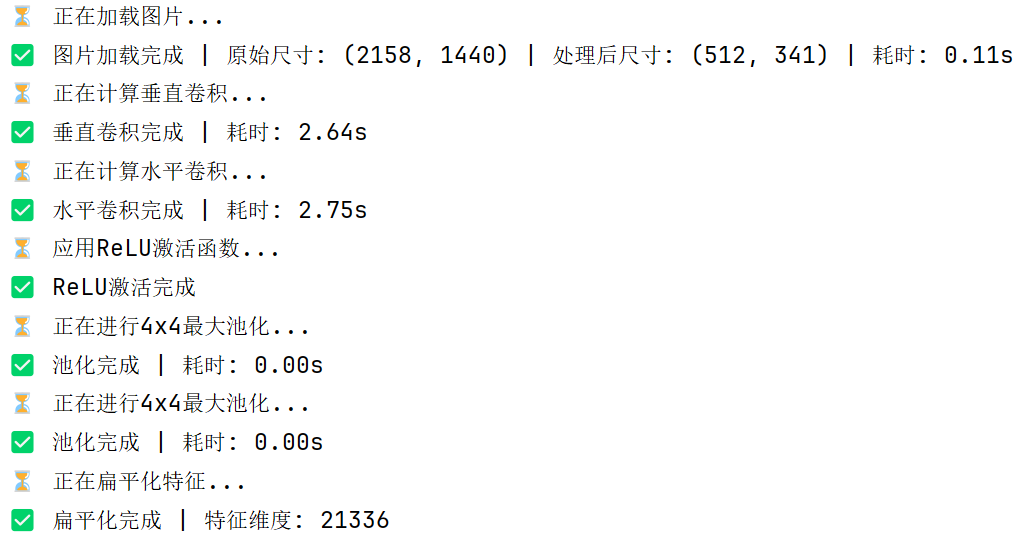

优化版

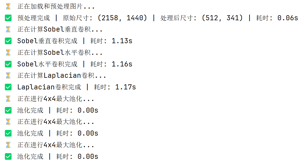
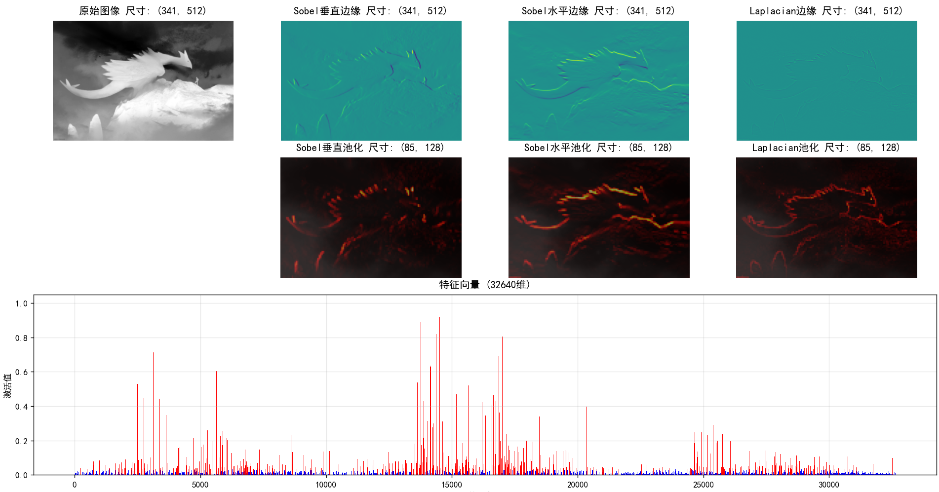
代码实现了一个增强版的图像特征提取流程，首先通过直方图均衡化和高斯滤波对图像进行增强预处理，然后使用三种不同的卷积核（Sobel垂直/水平边缘检测和Laplacian边缘增强）进行多尺度特征提取，并采用ReLU激活函数处理卷积结果；接着通过自适应最大池化降低特征维度，最后将多组特征归一化后拼接成综合特征向量。改进后的流程通过更专业的卷积核、反射填充边界和特征融合技术提升了特征提取效果，并采用优化的可视化布局同时展示原始图像、三类卷积结果、叠加显示的池化热力图以及最终的特征向量分布，完整呈现了从原始图像到高级特征的转换过程。

kernels = {'Sobel垂直': np.array([[-1, -2, 0, 2, 1],[-2, -4, 0, 4, 2],[-1, -2, 0, 2, 1]]) / 8,'Sobel水平': np.array([[-1, -2, -1],[-2, -4, -2],[0, 0, 0],[2, 4, 2],[1, 2, 1]]) / 8,'Laplacian': np.array([[0, 1, 0],[1, -4, 1],[0, 1, 0]])}

import numpy as np
import matplotlib.pyplot as plt
from PIL import Image
from skimage.util import view_as_blocks
from skimage import exposure
from scipy.ndimage import gaussian_filter
import time
import matplotlib# 设置中文字体
plt.rcParams['font.sans-serif'] = ['SimHei']  # Windows系统
plt.rcParams['axes.unicode_minus'] = Falsedef load_and_preprocess_image(image_path, max_size=512):"""加载图片并进行增强预处理"""print("⏳ 正在加载和预处理图片...")start_time = time.time()img = Image.open(image_path).convert('L')original_size = img.size# 修正后的尺寸计算行ratio = min(max_size / original_size[0], max_size / original_size[1])new_size = (int(original_size[0] * ratio), int(original_size[1] * ratio))img = img.resize(new_size, Image.LANCZOS)img_array = np.array(img, dtype=np.float32)img_array = exposure.equalize_hist(img_array)img_array = gaussian_filter(img_array, sigma=0.8)img_array = (img_array - img_array.min()) / (img_array.max() - img_array.min())img_array = 1 - img_arrayprint(f"✅ 预处理完成 | 原始尺寸: {original_size} | 处理后尺寸: {new_size} | 耗时: {time.time() - start_time:.2f}s")return img_arraydef enhanced_conv2d(image, kernel, operation_name=""):"""增强版卷积运算"""print(f"⏳ 正在计算{operation_name}卷积...")start_time = time.time()pad_h = kernel.shape[0] // 2pad_w = kernel.shape[1] // 2padded = np.pad(image, ((pad_h, pad_h), (pad_w, pad_w)), mode='reflect')h, w = image.shapek_h, k_w = kernel.shapeoutput = np.zeros_like(image)total_steps = hfor y in range(h):if y % 10 == 0 or y == total_steps - 1:print(f"  进度: {y + 1}/{total_steps}行", end='\r')for x in range(w):output[y, x] = np.sum(padded[y:y + k_h, x:x + k_w] * kernel)print(f"✅ {operation_name}卷积完成 | 耗时: {time.time() - start_time:.2f}s")return outputdef adaptive_maxpool(image, pool_size=4):"""自适应最大池化"""print(f"⏳ 正在进行{pool_size}x{pool_size}最大池化...")start_time = time.time()h, w = image.shapeh = h - h % pool_sizew = w - w % pool_sizeimage = image[:h, :w]blocks = view_as_blocks(image, (pool_size, pool_size))pooled = blocks.max(axis=2).max(axis=2)print(f"✅ 池化完成 | 耗时: {time.time() - start_time:.2f}s")return pooleddef visualize_enhanced_results(original, conv_results, pool_results, flattened):"""改进版可视化（优化布局）"""plt.figure(figsize=(16, 12))# 调整全局参数plt.rcParams['axes.titlepad'] = 8plt.subplots_adjust(left=0.05, right=0.95, bottom=0.05, top=0.92,wspace=0.15, hspace=0.3)# 创建2x4的网格布局gs = plt.GridSpec(3, 4, height_ratios=[1, 1, 1.5])# 1. 原始图像ax0 = plt.subplot(gs[0, 0])ax0.imshow(original, cmap='gray')ax0.set_title('原始图像 尺寸: {}'.format(original.shape))ax0.axis('off')# 2-4. 卷积结果titles = ['Sobel垂直边缘', 'Sobel水平边缘', 'Laplacian边缘']for idx, (name, conv) in enumerate(conv_results.items(), start=1):ax = plt.subplot(gs[0, idx])ax.imshow(conv, cmap='viridis', vmin=-1, vmax=1)ax.set_title('{} 尺寸: {}'.format(titles[idx - 1], conv.shape))ax.axis('off')# 5-7. 池化结果titles = ['Sobel垂直池化', 'Sobel水平池化', 'Laplacian池化']for idx, (name, pool) in enumerate(pool_results.items(), start=1):ax = plt.subplot(gs[1, idx])ax.imshow(original, cmap='gray')ax.imshow(pool, cmap='hot', alpha=0.5)ax.set_title('{} 尺寸: {}'.format(titles[idx - 1], pool.shape))ax.axis('off')# 8. 特征向量 (占据底部一整行)ax7 = plt.subplot(gs[2, :])colors = ['red' if x > np.mean(flattened) else 'blue' for x in flattened]ax7.bar(range(len(flattened)), flattened, color=colors, width=1.0)ax7.set_title('特征向量 ({}维)'.format(len(flattened)))ax7.set_xlabel('特征索引')ax7.set_ylabel('激活值')ax7.grid(True, alpha=0.3)plt.suptitle(' ', y=0.98, fontsize=16)plt.tight_layout()plt.show()def enhanced_feature_extraction(image_path, max_size=512, pool_size=4):"""增强版特征提取流程"""print("\n" + "=" * 50)print("🚀 开始增强版特征提取流程")print("=" * 50)original = load_and_preprocess_image(image_path, max_size)kernels = {'Sobel垂直': np.array([[-1, -2, 0, 2, 1],[-2, -4, 0, 4, 2],[-1, -2, 0, 2, 1]]) / 8,'Sobel水平': np.array([[-1, -2, -1],[-2, -4, -2],[0, 0, 0],[2, 4, 2],[1, 2, 1]]) / 8,'Laplacian': np.array([[0, 1, 0],[1, -4, 1],[0, 1, 0]])}conv_results = {}for name, kernel in kernels.items():conv = enhanced_conv2d(original, kernel, name)conv_results[name] = convrelu_results = {name: np.maximum(0, conv) for name, conv in conv_results.items()}combined_feature = np.max(list(relu_results.values()), axis=0)pool_results = {}for name, feature in relu_results.items():pool_results[name] = adaptive_maxpool(feature, pool_size)flattened = np.concatenate([pool.flatten() for pool in pool_results.values()])flattened = (flattened - np.min(flattened)) / (np.max(flattened) - np.min(flattened))visualize_enhanced_results(original, conv_results, pool_results, flattened)return {'original': original,'conv_results': conv_results,'pool_results': pool_results,'flattened_features': flattened}if __name__ == "__main__":image_path = "image.jpg"  # 替换为你的图片路径results = enhanced_feature_extraction(image_path)