AI大模型训练相关函数知识补充
1. 归一化函数
RMSNorm
import torch
import matplotlib.pyplot as pltclass RMSNorm(torch.nn.Module):def __init__(self, dim: int, eps: float = 1e-6):super().__init__()# eps防止取倒数之后分母为0self.eps = epsself.weight = torch.nn.Parameter(torch.ones(dim))def _norm(self, x):# torch.rsqrt是开平方并取倒数# x.pow(2)是平方# mean(-1)是在最后一个维度(即hidden特征维度)上取平均return x * torch.rsqrt(x.pow(2).mean(-1, keepdim=True) + self.eps)def forward(self, x):output = self._norm(x.float()).type_as(x)# weight是未居乘的可训练参数,即γreturn output * self.weight# 随机生成输入数据
batch_size = 8
hidden_dim = 16
x = torch.randn(batch_size, hidden_dim)# 实例化RMSNorm
norm = RMSNorm(dim=hidden_dim)# 前向传播
output = norm(x)# 可视化输入和输出
fig, axs = plt.subplots(1, 2, figsize=(10, 4))
axs[0].imshow(x.detach().numpy(), aspect='auto', cmap='viridis')
axs[0].set_title('Input')
axs[0].set_xlabel('Feature')
axs[0].set_ylabel('Batch')axs[1].imshow(output.detach().numpy(), aspect='auto', cmap='viridis')
axs[1].set_title('RMSNorm Output')
axs[1].set_xlabel('Feature')
axs[1].set_ylabel('Batch')plt.tight_layout()
plt.show() 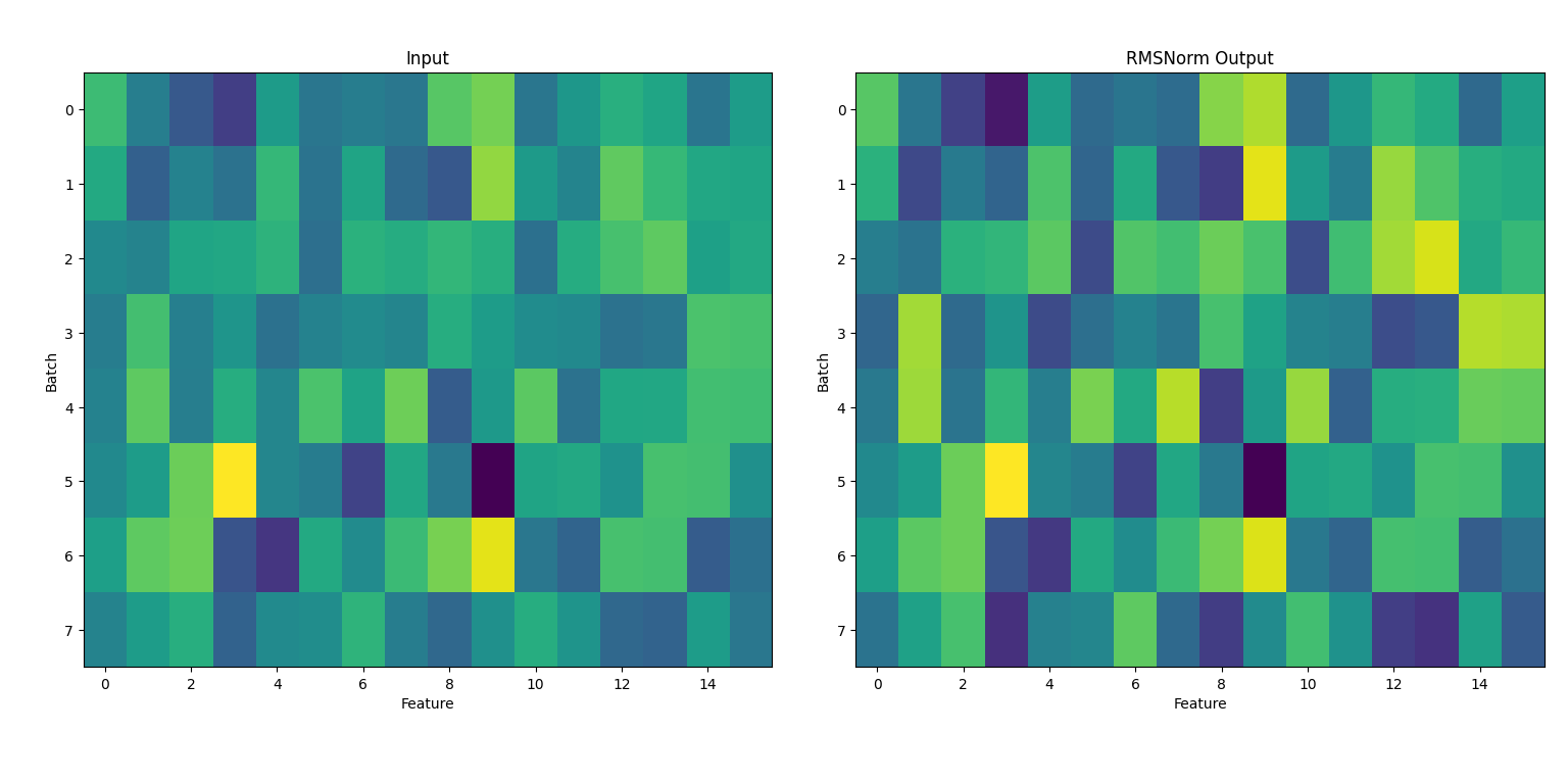
1. 输入数据(左图:Input)
- 内容:左侧的热力图展示了输入张量 x,其形状为 (8, 16),即8个batch,每个batch有16个特征。
- 颜色:颜色深浅代表数值大小,黄色为较大值,深蓝为较小值。
- 分布:由于 x 是用 torch.randn 随机生成的,整体呈现高斯分布,数值有正有负,分布较为均匀。
2. RMSNorm输出(右图:RMSNorm Output)
- 内容:右侧热力图展示了经过 RMSNorm 归一化后的输出。
- 归一化效果:
- RMSNorm 会对每个样本(batch的每一行)在特征维度上做归一化处理,使其均方根(RMS)接近1(受weight参数影响)。
- 归一化后,数值的极端差异被抑制,整体分布更集中,颜色分布更均匀。
- 可训练参数:RMSNorm中有一个可训练参数 weight(初始为全1),它会对归一化后的结果做缩放。由于未训练,当前输出和归一化结果一致。
3. 总结
- RMSNorm 能有效地将每个样本的特征归一化,提升模型训练的稳定性。
Swish函数
import numpy as np
import matplotlib.pyplot as plt# 标准Swish: x * sigmoid(x)
def swish(x):return x * (1 / (1 + np.exp(-x)))# 带参数β的Swish: x * sigmoid(βx)
def swish_beta(x, beta=1.5):return x * (1 / (1 + np.exp(-beta * x)))# SiLU(实际上就是Swish的β=1版本)
def silu(x):return x * (1 / (1 + np.exp(-x)))x = np.linspace(-6, 6, 200)plt.figure(figsize=(8, 5))
plt.plot(x, swish(x), label='Swish (β=1)')
plt.plot(x, swish_beta(x, beta=1.5), label='Swish (β=1.5)')
plt.plot(x, swish_beta(x, beta=0.5), label='Swish (β=0.5)')
plt.plot(x, silu(x), '--', label='SiLU (β=1)')plt.title('Comparison of Swish Variants')
plt.xlabel('x')
plt.ylabel('Activation')
plt.legend()
plt.grid(True)
plt.tight_layout()
plt.show()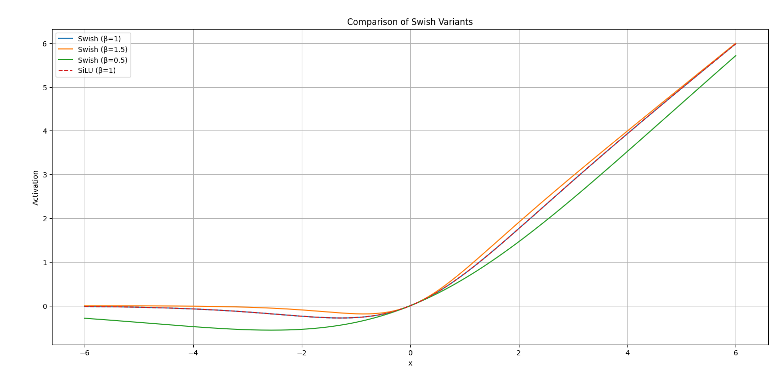
sinusoidal_position_embedding
import torch
import matplotlib.pyplot as pltdef sinusoidal_position_embedding(batch_size, nums_head, max_len, output_dim, device):# 生成位置序列 (max_len, 1)position = torch.arange(0, max_len, dtype=torch.float, device=device).unsqueeze(-1)# 生成ids (output_dim/2)ids = torch.arange(0, output_dim // 2, dtype=torch.float, device=device)# 计算thetatheta = torch.pow(10000, -2 * ids / output_dim)# 计算embeddings (max_len, output_dim/2)embeddings = position * theta# 拼接sin和cos (max_len, output_dim)embeddings = torch.stack([torch.sin(embeddings), torch.cos(embeddings)], dim=-1)embeddings = embeddings.view(max_len, output_dim)# 扩展到(batch_size, nums_head, max_len, output_dim)embeddings = embeddings.repeat(batch_size, nums_head, 1, 1)embeddings = embeddings.reshape(batch_size, nums_head, max_len, output_dim)return embeddings# 测试与可视化
if __name__ == "__main__":# 参数设置batch_size = 1nums_head = 1max_len = 50output_dim = 16device = torch.device('cpu')# 生成位置编码embeddings = sinusoidal_position_embedding(batch_size, nums_head, max_len, output_dim, device)# embeddings shape: (1, 1, max_len, output_dim)embeddings = embeddings[0, 0].detach().numpy() # 取第一个batch和head,shape: (max_len, output_dim)# 可视化:每一列代表一个维度,画出前几个维度随位置的变化plt.figure(figsize=(10, 6))for i in range(output_dim):plt.plot(range(max_len), embeddings[:, i], label=f'dim {i}')plt.title('Sinusoidal Position Embedding (each dim)')plt.xlabel('Position')plt.ylabel('Embedding Value')plt.legend(loc='upper right', ncol=2, fontsize=8)plt.tight_layout()plt.show() 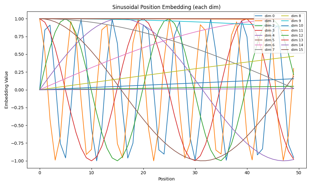
RoPE 函数:
为 Transformer 中的 query(q)和 key(k)向量引入“旋转式”绝对/相对位置信息,使模型能够感知序列中各 token 的顺序和相对距离。
import torch
import matplotlib.pyplot as plt
from sinusoidal_position_embedding import sinusoidal_position_embeddingdef RoPE(q, k, visualize=False):"""Rotary Position Embedding (RoPE) for query and key tensors.Args:q: Tensor of shape (batch_size, num_heads, seq_len, head_dim)k: Tensor of shape (batch_size, num_heads, seq_len, head_dim)visualize: If True, visualize before/after RoPE for the first token and headReturns:Tuple of rotated (q, k)"""batch_size, num_heads, seq_len, head_dim = q.shapepos_emb = sinusoidal_position_embedding(batch_size, num_heads, seq_len, head_dim, q.device)sin_pos = pos_emb[..., ::2]cos_pos = pos_emb[..., 1::2]sin_pos = sin_pos.repeat_interleave(2, dim=-1)cos_pos = cos_pos.repeat_interleave(2, dim=-1)def apply_rope(x, sin_pos, cos_pos):x1 = x[..., ::2]x2 = x[..., 1::2]x_rotated = torch.stack([-x2, x1], dim=-1).reshape_as(x)return x * cos_pos + x_rotated * sin_posq_before = q.clone().detach()k_before = k.clone().detach()q = apply_rope(q, sin_pos, cos_pos)k = apply_rope(k, sin_pos, cos_pos)if visualize:# 可视化第一个 batch、head,所有 token 的前4个维度 before/afterplt.figure(figsize=(12, 6))for d in range(4):q0 = q_before[0, 0, :, d].cpu().numpy()q1 = q[0, 0, :, d].cpu().numpy()plt.subplot(2, 4, d+1)plt.plot(range(len(q0)), q0, label='before')plt.plot(range(len(q1)), q1, label='after')plt.title(f'q dim {d}')if d == 0:plt.ylabel('Value')plt.xlabel('Token pos')plt.legend(fontsize=8)# 差值diff = q1 - q0plt.subplot(2, 4, d+5)plt.plot(range(len(diff)), diff, label='after-before', color='purple')plt.title(f'q diff dim {d}')if d == 0:plt.ylabel('Delta')plt.xlabel('Token pos')plt.legend(fontsize=8)plt.tight_layout()plt.suptitle('RoPE effect on q (first 4 dims, all tokens)', y=1.02)plt.show()return q, kif __name__ == "__main__":# 测试与可视化batch_size = 1num_heads = 1seq_len = 10head_dim = 16device = torch.device('cpu')torch.manual_seed(42)q = torch.randn(batch_size, num_heads, seq_len, head_dim, device=device)k = torch.randn(batch_size, num_heads, seq_len, head_dim, device=device)q_rope, k_rope = RoPE(q, k, visualize=True)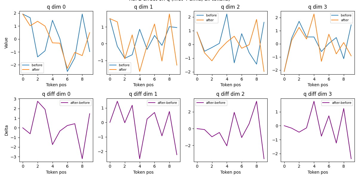
1. 介绍
- Transformer 原生结构对序列顺序不敏感,需要人为加入“位置信息”。
- 常见做法有:加法位置编码(如 BERT)、正弦位置编码(如原始 Transformer)、RoPE(旋转式位置编码,常用于 Llama、GLM 等新模型)。
2. RoPE 的原理
- RoPE 不是简单地把位置编码加到输入上,而是将每个 token 的向量在高维空间中“旋转”一个与其位置相关的角度。
- 这种旋转操作可以让注意力分数(q·k)天然地包含 token 之间的相对位置信息。
- 旋转的角度由正弦/余弦函数生成,周期性强,适合捕捉序列结构。
3. 函数输入输出
- 输入:q, k,形状为 (batch_size, num_heads, seq_len, head_dim) 的张量。
- 输出:经过 RoPE 旋转后的 q, k,形状不变。
4. 实际效果
- 经过 RoPE 后,q/k 向量的每一维都被“周期性旋转”,这样模型在计算注意力时能区分不同 token 的顺序和距离。
- 这种方式比传统位置编码更适合大模型、长序列,且支持相对位置感知。