matlab解常微分方程常用数值解法2:龙格库塔方法
总结和记录一下matlab求解常微分方程常用的数值解法,本文将介绍龙格库塔方法(Runge-Kutta Method)。
龙格库塔迭代的基本思想是:
x k + 1 = x k + a k 1 + b k 2 x_{k+1}=x_{k}+a k_{1}+b k_{2} xk+1=xk+ak1+bk2
k 1 = h f ( x k , t k ) and k 2 = h f ( x k + B 1 k 1 , t k + A 1 h ) k_{1}=h f\left(x_{k},t_{k} \right) \quad \text { and } \quad k_{2}=h f\left(x_{k}+B_{1}k_{1},t_{k}+A_{1} h \right) k1=hf(xk,tk) and k2=hf(xk+B1k1,tk+A1h)
其中 a , b , A 1 , B 1 a,b,A_1,B_1 a,b,A1,B1是未知的,我们进行推导。
首先对 f ( x + k , t + h ) f(x+k,t+h) f(x+k,t+h)进行泰勒展开:
f ( x + k , t + h ) = f ( x , t ) + ( k f x + h f t ) + 1 2 ( k 2 f x x + 2 k h f x t + h 2 f t t ) + 1 6 ( k 3 f x x x + 3 k 2 h f x x t + 3 k h 2 f x t t + h 3 f t t t ) + ⋯ \begin{aligned} f(x+k, t+h) & =f(x, t)+\left(k f_{x}+h f_{t}\right)+\frac{1}{2}\left(k^{2} f_{xx}+2 k h f_{xt }+h^{2} f_{tt}\right) \\ & +\frac{1}{6}\left(k^{3} f_{xxx}+3 k^{2} h f_{xxt}+3 k h^{2} f_{xtt}+h^{3} f_{ttt}\right)+\cdots \end{aligned} f(x+k,t+h)=f(x,t)+(kfx+hft)+21(k2fxx+2khfxt+h2ftt)+61(k3fxxx+3k2hfxxt+3kh2fxtt+h3fttt)+⋯
利用泰勒展开我们展开 k 2 k_2 k2:
k 2 = h f [ x k + B 1 h f ( x k , t k ) , t k + A 1 h ] = h [ f ( x k , t k ) + ( B 1 h f f x + A 1 h f t ) ] = h f + A 1 h 2 f t + B 1 h 2 f f x , \begin{aligned} k_{2} & =h f\left[x_{k}+B_1 h f\left( x_{k},t_{k}\right),t_{k}+A_{1} h\right] \\ & =h\left[f\left(x_{k},t_{k} \right)+\left(B_{1} h f f_{x}+A_{1} h f_{t}\right)\right] \\ & =h f+A_{1} h^{2} f_{t}+B_{1} h^{2} f f_{x}, \end{aligned} k2=hf[xk+B1hf(xk,tk),tk+A1h]=h[f(xk,tk)+(B1hffx+A1hft)]=hf+A1h2ft+B1h2ffx,
上式中的 f f f为 f ( x k , t k ) f(x_k,t_k) f(xk,tk),我们将上式代回到最开始的式子 x k + 1 = x k + a k 1 + b k 2 x_{k+1}=x_{k}+a k_{1}+b k_{2} xk+1=xk+ak1+bk2得到(*)式
x k + 1 = x k + ( a + b ) h f + ( A 1 b f t + B 1 b f f x ) h 2 ( ∗ ) x_{k+1}=x_{k}+(a+b) h f+\left(A_{1} b f_{t}+B_{1} b f f_{x}\right) h^{2}\quad\quad(*) xk+1=xk+(a+b)hf+(A1bft+B1bffx)h2(∗)
对应于二阶泰勒展式:
x k + 1 = x k + h x k ′ + 1 2 h 2 x k ′ ′ x_{k+1}=x_{k}+h x_{k}^{\prime}+\frac{1}{2} h^{2} x_{k}^{\prime \prime} xk+1=xk+hxk′+21h2xk′′
对于微分方程我们知道 x ′ = f ( x , t ) x^{\prime}=f(x, t) x′=f(x,t),于是对 t t t求二阶导数:
x ′ ′ = f t + f x x ′ = f t + f f x x^{\prime \prime}=f_{t}+f_{x} x^{\prime}=f_{t}+f f_{x} x′′=ft+fxx′=ft+ffx
于是有:
x k + 1 = x k + h f + 1 2 h 2 ( f t + f f x ) x_{k+1}=x_{k}+h f+\frac{1}{2} h^{2}\left(f_{t}+f f_{x}\right) xk+1=xk+hf+21h2(ft+ffx)
对比(*)式我们有:
a + b = 1 , A 1 b = 1 2 , and B 1 b = 1 2 . a+b=1, A_{1} b=\frac{1}{2}, \quad \text { and } \quad B_{1} b=\frac{1}{2} \text {. } a+b=1,A1b=21, and B1b=21.
如果我们取 a = b = 1 2 a=b=\frac{1}{2} a=b=21,那么 A 1 = B 1 = 1 A_1=B_1=1 A1=B1=1,为二阶的龙哥库塔算法。其形式和改进的欧拉法一致:
x k + 1 = x k + 1 2 ( k 1 + k 2 ) x_{k+1}=x_{k}+\frac{1}{2}\left(k_{1}+k_{2}\right) xk+1=xk+21(k1+k2)
从二阶的出发,我们可以得到改进的一套更好的框架,一个常用的龙哥库塔方法是四阶的:
x k + 1 = x k + 1 6 ( k 1 + 2 k 2 + 2 k 3 + k 4 ) , x_{k+1}=x_{k}+\frac{1}{6}\left(k_{1}+2 k_{2}+2 k_{3}+k_{4}\right) \text {, } xk+1=xk+61(k1+2k2+2k3+k4),
其中:
k 1 = h f ( x k , t k ) k 2 = h f ( x k + 1 2 k 1 , t k + 1 2 h ) k 3 = h f ( x k + 1 2 k 2 , t k + 1 2 h ) k 4 = h f ( x k + k 3 , t k + h ) \begin{aligned} &k_{1}=h f\left(x_{k},t_{k} \right) \\ &k_{2}=h f\left(x_{k}+\frac{1}{2} k_{1},t_{k}+\frac{1}{2} h \right) \\ &k_{3}=h f\left(x_{k}+\frac{1}{2} k_{2},t_{k}+\frac{1}{2} h \right) \\ &k_{4}=h f\left(x_{k}+k_{3},t_{k}+h\right) \end{aligned} k1=hf(xk,tk)k2=hf(xk+21k1,tk+21h)k3=hf(xk+21k2,tk+21h)k4=hf(xk+k3,tk+h)
例子
x ′ = x + t , x ( 0 ) = 1 x^{\prime}=x+t, \quad x(0)=1 x′=x+t,x(0)=1
clc
clear
% 测试4个不同的步长
test_times = 3;
h_test = [0.10, 0.05, 0.01];%根据步长数改变% 保存时间、差分时间和步长
h_res=ones(1,test_times);
t_res=cell(1,test_times);%时间
tplot_res=cell(1,test_times);%差分的时间,比时间长度少1
% 保存两种数值方法和解析解的计算结果
x_rk_res=cell(1,test_times);
x_exact_res=cell(1,test_times);
% 保存误差
diff_res=cell(1,test_times);for i = 1:test_times
% 设置步长间隔和步长数h = h_test(i);n = 10/h;
% 设置初始条件t=zeros(n+1,1); t(1) = 0;x_rk=zeros(n+1,1); x_rk(1) = 1;x_exact=zeros(n+1,1); x_exact(1) = 1;
% 设置龙哥库塔方法误差存放向量(和精确解比较)diff = zeros(n,1); tplot = zeros(n,1);
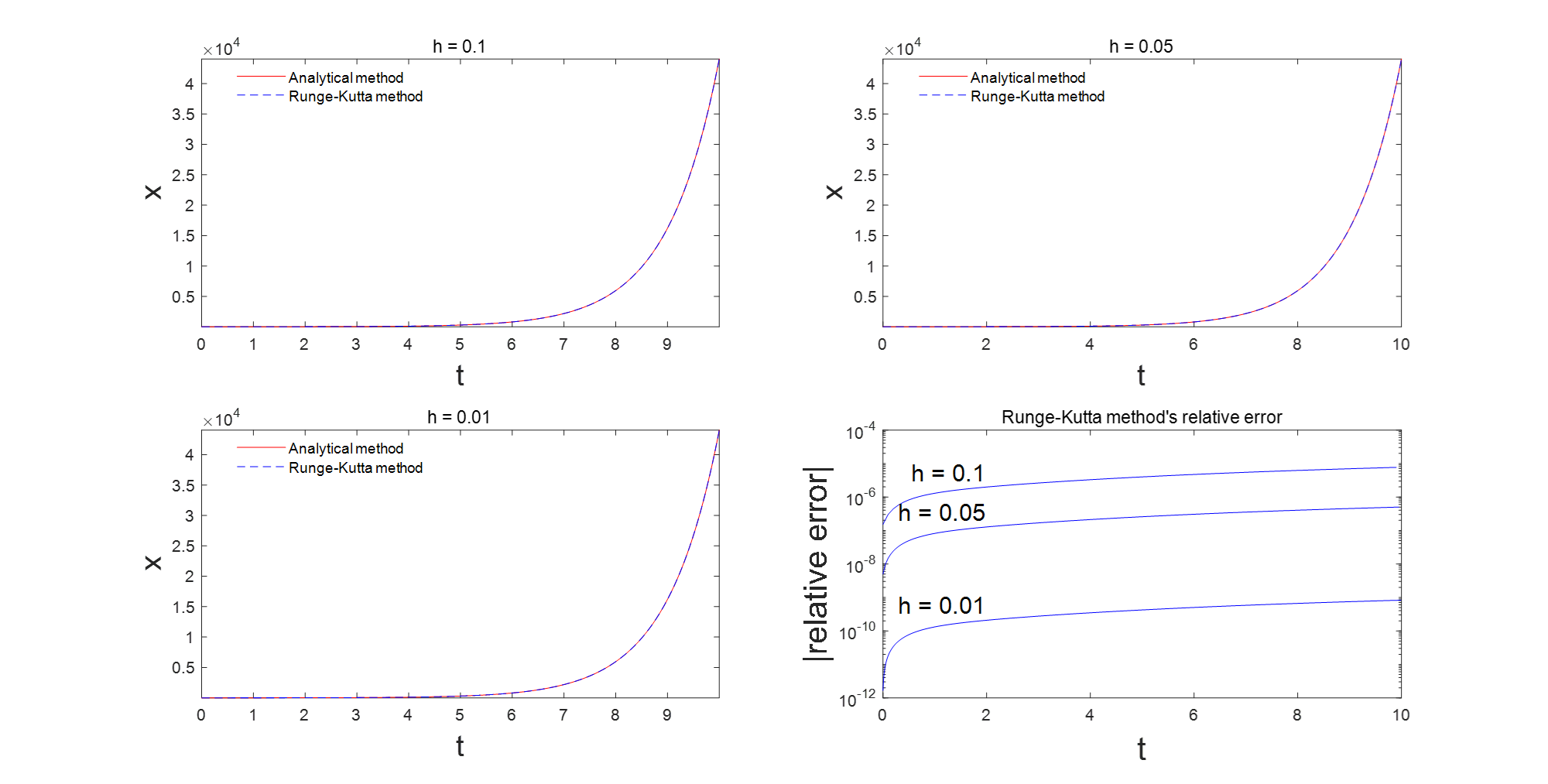
% 定义微分方程f = @(tt,xx)(xx+tt);for k = 1:nx_local = x_rk(k); t_local = t(k);k1 = h * f(t_local,x_local);k2 = h * f(t_local + h/2,x_local + k1/2);k3 = h * f(t_local + h/2,x_local + k2/2);k4 = h * f(t_local + h,x_local + k3);t(k+1) = t_local + h;x_rk(k+1) = x_local + (k1+2*k2+2*k3+k4) / 6;x_exact(k+1) = 2*exp(t(k+1)) - t(k+1) - 1;tplot(k) = t(k);diff(k) = x_rk(k+1) - x_exact(k+1);diff(k) = abs(diff(k) / x_exact(k+1));enddiff_res{i}=diff;tplot_res{i}=tplot;h_res(i)=h;x_rk_res{i}=x_rk;x_exact_res{i}=x_exact;t_res{i}=t;
endfigure
% 不同步长下的解析解和龙哥库塔法的结果
for i=1:test_timessubplot(2,2,i)plot(t_res{i},x_exact_res{i},'r-',t_res{i},x_rk_res{i},'b--')xlabel('t','Fontsize',18)ylabel('x','Fontsize',18)legend({'Analytical method','Runge-Kutta method'},'Location','best')legend boxoff;title(['h = ',num2str(h_res(i))]);axis tight
end% 相对误差图
subplot(2,2,4)
for i = 1:test_timessemilogy(tplot_res{i},diff_res{i},'b-')hold onnum1 = 2; num2 = 2/h_test(i);text(num1,diff_res{i}(num2),['h = ',num2str(h_res(i))],'Fontsize',15,...'HorizontalAlignment','right',...'VerticalAlignment','bottom')
end
xlabel('t','Fontsize',20)
ylabel('|relative error|','Fontsize',20)
title('Runge-Kutta method''s relative error')
可以看到使用龙格库塔法,步长 h = 0.1 h=0.1 h=0.1精度就已经很高了。