当前位置：首页 > news >正文

数据分析与预处理常用的图和代码

news 2025/7/6 21:15:07

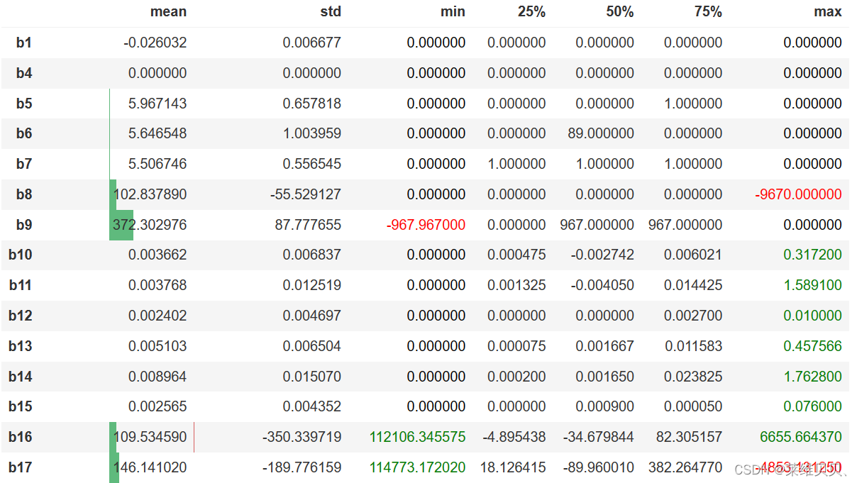
1.训练集和测试集统计数据描述之间的差异作图：

def diff_color(x):color = 'red' if x<0 else ('green' if x > 0 else 'black')return f'color: {color}'(train.describe() - test.describe())[features].T.iloc[:,1:].style\.bar(subset=['mean', 'std'], align='mid', color=['#d65f5f', '#5fba7d'])\.applymap(diff_color, subset=['min', 'max'])

在这里插入图片描述
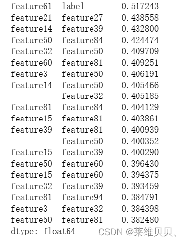
2. 特征之间的相似性排序

# 计算相关系数矩阵
corr_matrix = train_df.corr()
# 将对角线及以下部分置为 NaN
corr_matrix.where(np.triu(np.ones(corr_matrix.shape), k=1).astype(np.bool), inplace=True)
# 对相关系数矩阵进行排序
corr_sorted = corr_matrix.stack().sort_values(ascending=False)
# 打印排序后的相关系数
print(corr_sorted[:20])

在这里插入图片描述

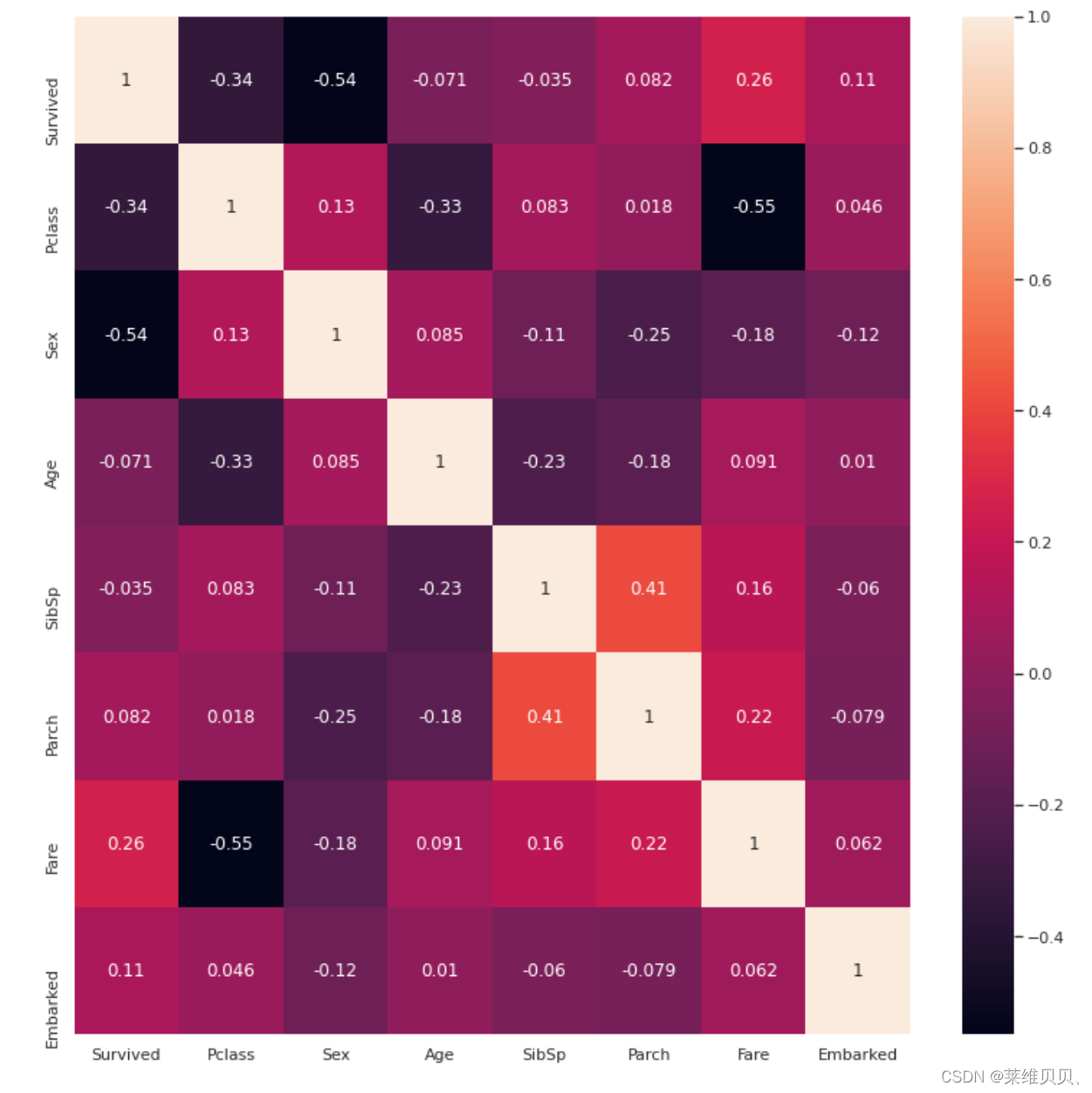
# 相似度图
sns.set(rc={'figure.figsize':(13,13)})
ax = sns.heatmap(train.corr(), annot=True)
# 筛选相似度
corr = train.corr()
sns.heatmap(corr[((corr >= 0.3) | (corr <= -0.3)) & (corr != 1)], annot=True, linewidths=.5, fmt= '.2f')
plt.title('Configured Corelation Matrix');

在这里插入图片描述

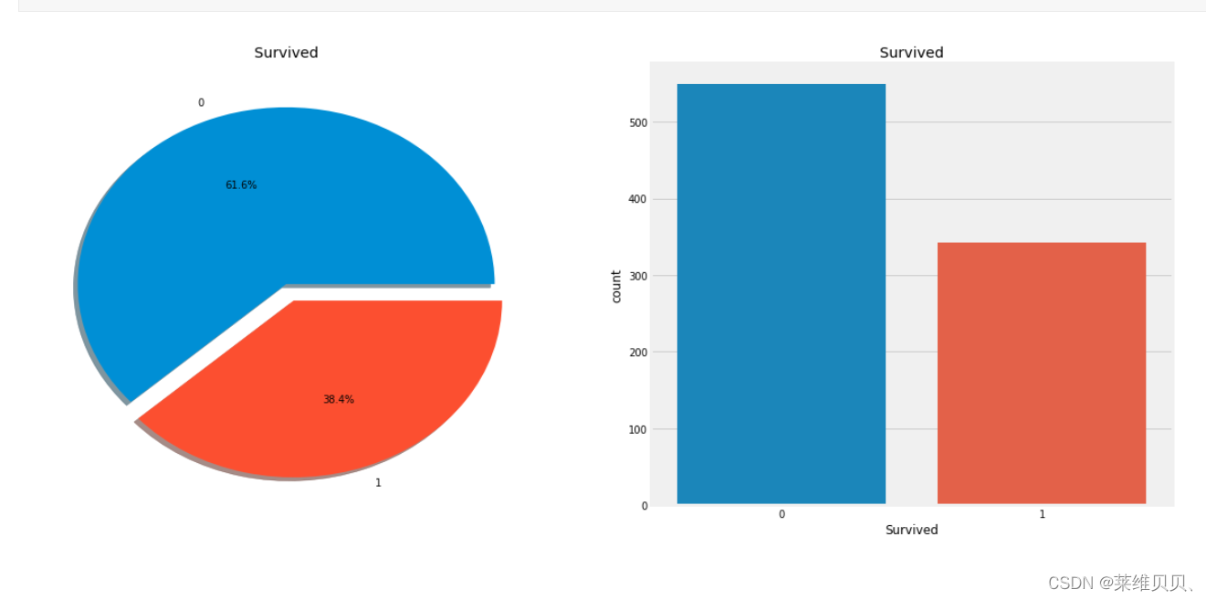
3.画标签比例图

f,ax=plt.subplots(1,2,figsize=(18,8))
data['Survived'].value_counts().plot.pie(explode=[0,0.1],autopct='%1.1f%%',ax=ax[0],shadow=True)
ax[0].set_title('Survived')
ax[0].set_ylabel('')
sns.countplot(x='Survived',data=data,ax=ax[1])
ax[1].set_title('Survived')
plt.show()

在这里插入图片描述
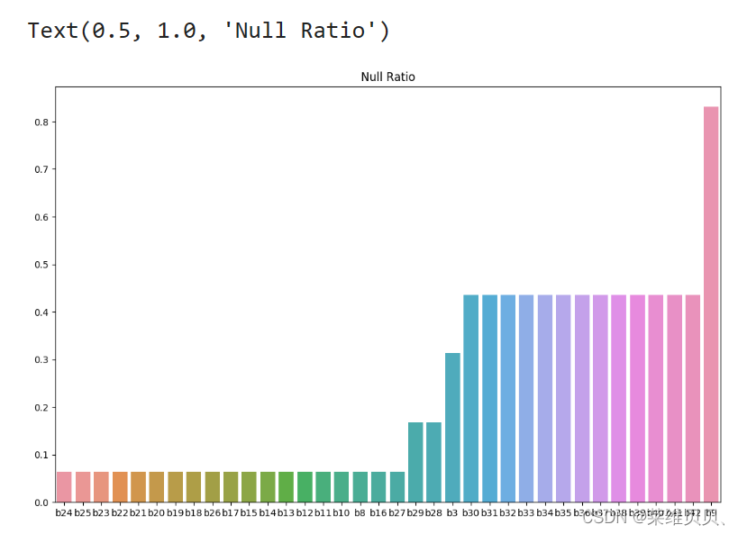
4. 查看缺失以及可视化

# 查看缺失率大于50%的特征
have_null_fea_dict = (train.isnull().sum()/len(train)).to_dict()
fea_null_moreThanHalf = {}
for key,value in have_null_fea_dict.items():if value > 0.5:fea_null_moreThanHalf[key] = value
fea_null_moreThanHalf
# nan可视化
f,ax = plt.subplots(1,2,figsize=(28,8),facecolor='w')# 设置画布大小，分辨率，和底色
missing = train.isnull().sum()/len(train)
missing = missing[missing > 0]
missing.sort_values(inplace=True)
missing.plot.bar(ax=ax[0])
sns.barplot(x=missing.index,y=missing.values,ax=ax[0])
ax[0].tick_params(axis='x', rotation=0)
ax[0].set_title('Null Ratio')

在这里插入图片描述
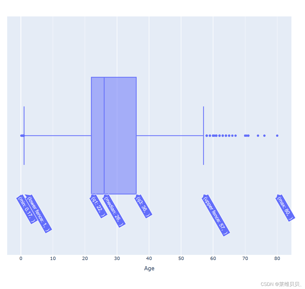
5.异常值查看以及可视化

sns.factorplot(x = "Sex", y = "Age", data = train_df, kind = "box")
plt.show()

在这里插入图片描述

5. 类别特征数据分析

# 教育情况
plt.rcParams['font.sans-serif'] = ['Songti SC']
f,ax=plt.subplots(1,2,figsize=(18,8))
sns.countplot(x='b3',hue='label',data=train,ax=ax[0])
ax[0].set_title('Degree:Staging vs Not Staging')
ax[0].set_xlabel("Degree")
train[['b3','label']].groupby(['b3']).mean().plot.bar(ax=ax[1])
for p in ax[1].patches:ax[1].annotate(f'\n{round(p.get_height(),2)}', (p.get_x()+0.15, p.get_height()+0.001), color='black', size=12)
ax[1].tick_params(axis='x', rotation=0)
ax[1].set_title('Staging Ratio')
ax[1].set_xlabel("Degree")
plt.show()

在这里插入图片描述
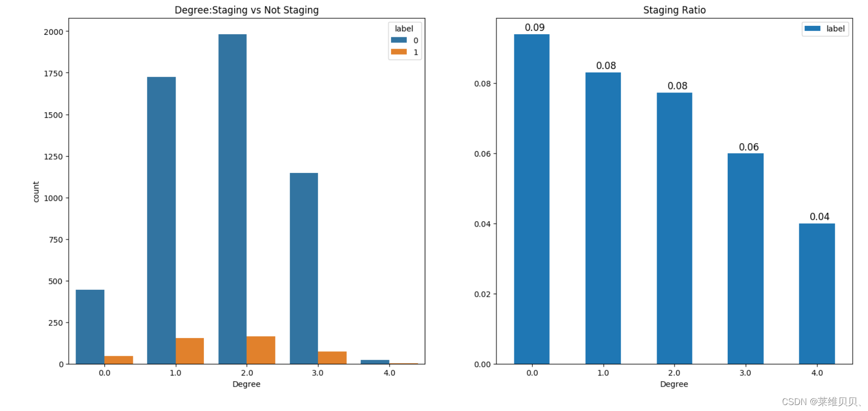
（ps：从图中可以发现，随着学历的提高，同学历情况下，选择分期付款占比越来越小）

6.数据分布情况查看

（ps：查看那些特征，可以将不同类别的标签数据分开）

def plot_feature_distribution(df1, df2,df3, label1, label2, label3,  features):i = 0sns.set_style('whitegrid')plt.figure()fig, ax = plt.subplots(11,10,figsize=(18,22))for feature in features:print(feature)i += 1plt.subplot(11,10,i)try:sns.distplot(df1[feature], hist=False,label=label1)sns.distplot(df2[feature], hist=False,label=label2)sns.distplot(df3[feature], hist=False,label=label3)except:print(feature)plt.xlabel(feature, fontsize=9)locs, labels = plt.xticks()plt.tick_params(axis='x', which='major', labelsize=6, pad=-6)plt.tick_params(axis='y', which='major', labelsize=6)plt.show();
t0 = train_df.loc[train_df['label'] == 0]
t1 = train_df.loc[train_df['label'] == 1]
t2 = train_df.loc[train_df['label'] == 2]features = train_df.columns.values[1:106]
plot_feature_distribution(t0, t1,t2,  '0', '1','2', features)

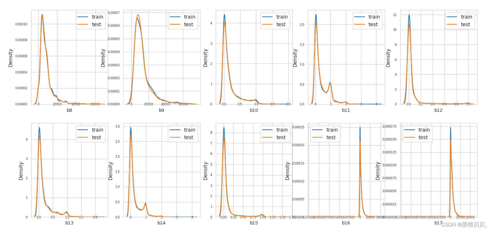
7.训练数据和测试数据分布查看
（ps：查看那些特征，在训练数据和测试数据上存在较大差异，如果存在，删去）

def plot_feature_distribution(df1, df2, label1, label2, features):i = 0sns.set_style('whitegrid')plt.figure()fig, ax = plt.subplots(11,10,figsize=(16,32))for feature in features:i += 1plt.subplot(11,10,i)sns.distplot(df1[feature], hist=False,label=label1)sns.distplot(df2[feature], hist=False,label=label2)plt.xlabel(feature, fontsize=9)locs, labels = plt.xticks()plt.tick_params(axis='x', which='major', labelsize=6, pad=-6)plt.tick_params(axis='y', which='major', labelsize=6)plt.legend()plt.show()
features = train_df.columns.values[1:106]
plot_feature_distribution(train_df, test_df, 'train', 'test', features)

在这里插入图片描述
8.RFECV最优特征选取
利用递归的方法进行，特征筛选

from sklearn.feature_selection import RFECV# 定义一个LightGBM分类器
clf = lgb.LGBMClassifier()
# 定义RFECV选择器
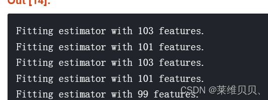
rfecv_selector = RFECV(estimator=clf, n_jobs=8,verbose=1,step=2, cv=2, scoring='accuracy')# 使用RFECV选择器训练数据
rfecv_selector.fit(train_x[features], train_y)
print('Finished')

在这里插入图片描述

# 得到选择后的特征子集
max_x = np.argmax(rfecv_selector.grid_scores_[1:])
max_y =  np.max(rfecv_selector.grid_scores_[1:])# 绘制特征数量与交叉验证分数之间的关系曲线
plt.figure(figsize=(12,6))
plt.title('RFECV with LightGBM')
plt.xlabel('Number of features selected')
plt.ylabel('Cross validation score (accuracy)')
plt.plot([103-2*i for i in range(51)], rfecv_selector.grid_scores_[1:][::-1])plt.annotate(f'max: ({93}, {max_y:.2f})', xy=(max_x+48, max_y), xytext=(max_x+48, max_y),arrowprops=dict(facecolor='red',width=10, shrink=0.05))
plt.show()