基于transformer的目标检测——匈牙利匹配算法
目前目标检测系列分为基于卷积神经网络(CNN)系列和基于transformer方法系列。对于卷积系列我个人也学习了很多,而对于基于transformer系列的也开始在了解。所以我打算起一个专栏,专门对自己知识的盲区进行扫盲。所以这个系列的文章,也是想到什么总结什么。
最近在使用C++复现DEIM的代码。同时也是了解到Hungarian Matching算法。这一篇就从匈牙利匹配开始吧。注意我这里只介绍与DEIM中用到的代码相关的逻辑。至于更深层次的或者其他的我暂时不做了解。
匈牙利匹配(Hungarian Matching)在深度学习目标检测中主要用于解决目标检测框(bounding box)与真实标注框(Ground truth)之间的最优匹配问题,尤其是在多目标场景下(如DETR等模型)。我会先简单的了解一下用到的基础原理和深度学习的理论。
1,匈牙利匹配算法原理
匈牙利匹配算法(Hungarian Algorithm)是一种解决二分图最小权匹配问题的多项式时间算法。其时间复杂度是O(N**3),在目标检测中:
- 1,将预测框和真实框视为二分图的两部分
- 2,需要找到预测框和真实框之间的最优一对一匹配
数字形式化:对于N个预测框和M个真实框(M≤N),定义代价矩阵C∈ℝ^(N×M),其中Cij表示第i个预测框与第j个真实框的匹配代价。目标是找到排列σ∈𝔖_N使得总代价最小:

概念太抽象的话,我这个来一个图。假设你有三个预测框(P1, P2, P3)和三个真实框(G1, G2, G3)。如下:
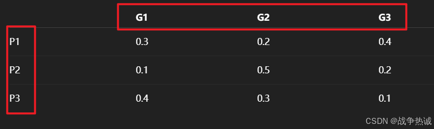
匈牙利算法会找到一个最优的分配方式(比如P1->G2, P2->G1, P3->G3),使得总代价最小。我们计算了预测和真实之间的代价矩阵,默认情况下匈牙利算法返回的是最优解,即最小代价。
下面来以一个距离的例子来说一下其理论原理。
1.1 问题背景:任务分配问题
假设我们有:
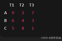
3名工人:A,B,C
3项任务:T1, T2, T3
每个工人完成一项任务的成本(花费)如下:
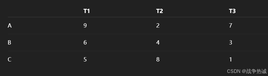
目标:我们希望每个工人只做一项任务,并且任务每个只能被一个人做,使得总成本最低。
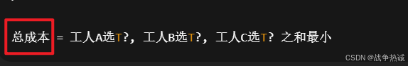
1.2 目标:找出最优分配
对于上面的3*3的表,问题就是找出一种一一对应的分配,使得总成本最低:
最简单的方法就是暴力法:暴力法会尝试所有3 !=6种组合。匈牙利算法可以在线性规划中高效的求解出最优组合,时间复杂度为O(n^3)。
1.3 匈牙利算法原理简化解释
如果我们使用匈牙利算法,如何做呢? 下面是其步骤
step1:行/列减操作(简化问题)
每一行减去最小值:让每行都有一个0
然后每一列再减去最小值:让每列也都有一个0
(这一步不会改变最优匹配的位置,但是方便之后找0)
step2:寻找覆盖所有0的最少行/列数
找出矩阵中所有的0
用尽量少的横线/竖线覆盖所有0 (如果能用n条线覆盖所有0(即方针维度),说明最优匹配已找到)。否则:
在未覆盖区域中找最小值
修改矩阵值(调整0的布局)
重复该步骤直到找到最优匹配
step3:进行匹配
在只含0的位置进行分配(不能同行或同列),最后得到最优分配方案。
step4:数学推理
原始代价矩阵,如下(就是上面的数字)
按照步骤1:第一步行减:(每行减去最小值,让每行都有一个0)
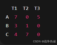
第二步列减:(让每一列再减去最小值,这样每列也有一个0)
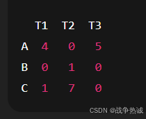
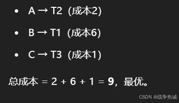
然后尝试选择不冲突的0来匹配每个人,最终得到一个最优匹配,比如:
1.4 匈牙利匹配算法的python实现-linear_sum_assignment
python中的SciPy库提供了linear_sum_assignment函数,用于解决线性分类问题(Linear Sum Assigment Problem, LSAP),即经典的二分图最小权匹配问题。他实现了匈牙利算法(Hungarian Algorithm),用于在给定的代价矩阵中找到最优的一对一匹配,使得总代价最小。
Scipy的linear_sum_assignment的函数签名:
from scipy.optimize import linear_sum_assignment
row_ind, col_ind = linear_sum_assignment(cost_matrix, maximize=False)输入:
cost_matrix:n x m的代价矩阵(n任务,m工人)。maximize:若为True,则求解最大权匹配(如最大化IoU)。
输出:
row_ind:匹配的行索引(任务ID)。col_ind:匹配的列索引(工人ID)。
示例:
import numpy as np
from scipy.optimize import linear_sum_assignment# 代价矩阵:3个预测框 vs 2个真实框(行列可不等)
cost_matrix = np.array([[1, 2],  # 预测框1与真实框1/2的代价[3, 4],  # 预测框2与真实框1/2的代价[5, 6]   # 预测框3与真实框1/2的代价
])# 找到最小代价匹配
row_ind, col_ind = linear_sum_assignment(cost_matrix)
print("匹配结果:", row_ind, col_ind)  # 输出:[0, 1], [0, 1] → 预测框1←→真实框1, 预测框2←→真实框2
print("总代价:", cost_matrix[row_ind, col_ind].sum())  # 输出:1 + 4 = 5
2,匈牙利匹配在目标检测的应用
我们知道目标检测模型会生成大量预测框(如YOLO的Anchor Boxes或DETR的预测集合),但需要确定那些预测框对应哪些真实标注框。所以匹配的目标就是:最小化预测与真实值之间的整体差异(如位置误差,分类误差)。
而匈牙利匹配的核心思想就是二分图匹配:将预测框和真实框视为二分图的两部分,通过计算他们之间的代价(cost),找到最优的一对一匹配。
2.1 实例:深度学习演示匈牙利匹配算法过程
在深度学习目标检测中,比如每张图预测了多个目标:pred_boxes(模型预测的框),gt_boxes(标注的真实框)。我们使用匈牙利匹配,找出哪个预测最匹配哪个真实框(一对一)
当然匹配标注中可能包含:分类损失,L1框差异,GIOU框重叠程度。然后利用这些匹配关系来监督训练。
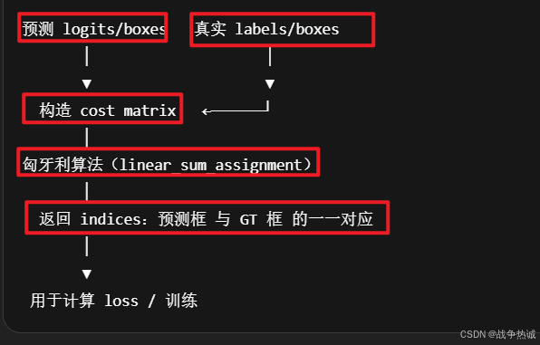
如上流程:其内容包括:
模拟预测框(pred_logits和pred_boxes)和目标框(targets)
构建 cost matrix(分类cost + L1 box cost + GIOU cost)
使用匈牙利算法找出最优匹配对
step1:模拟数据构建
假设有一张图(batch=1),模型输出了3个预测框,Ground Truth有两个目标。模拟预测(outputs):
# 分类 logits(预测框对3个类别的分数)
pred_logits = torch.tensor([[[2.0, 0.1, 0.1],    # 第一个预测框:class 0[0.1, 2.0, 0.1],    # 第二个预测框:class 1[0.1, 0.1, 2.0]]    # 第三个预测框:class 2
])  # shape: [1, 3, 3]# 预测框(中心点坐标 cx, cy, 宽 w,高 h)格式
pred_boxes = torch.tensor([[[0.5, 0.5, 1.0, 1.0],   # box 1[2.0, 2.0, 1.0, 1.0],   # box 2[3.0, 3.0, 1.0, 1.0]]   # box 3
])  # shape: [1, 3, 4]
模拟Ground truth:
targets = [{"labels": torch.tensor([0, 2]),                 # 第一个GT是类0,第二个GT是类2"boxes": torch.tensor([[0.6, 0.6, 1.0, 1.0],     # GT1[3.1, 3.1, 1.0, 1.0]])    # GT2
}]
step2:计算Cost matrix
1,分类cost:我们用softmax后的概率来计算 cost_class=-log(p[class]) 即负对数似然。
from torch.nn.functional import softmax
import torchprobs = softmax(pred_logits, dim=-1)[0]  # shape: [3, 3]
print("分类概率:\n", probs)
# GT标签是[0, 2],我们取每个预测框对 class 0 和 class 2 的概率
cost_class = -probs[:, [0, 2]]
print("分类代价 (负log概率):\n", cost_class)
输出类似:
分类概率:
tensor([[0.8438, 0.0781, 0.0781],[0.0781, 0.8438, 0.0781],[0.0781, 0.0781, 0.8438]])cost_class:
tensor([[-0.1696, -2.5494],   # 预测框1与GT0、GT2[-2.5494, -2.5494],   # 预测框2[-2.5494, -0.1696]])  # 预测框3
2,L1 box cost:
from torch.cdist import cdist# 展平预测框和 GT 框
boxes_pred = pred_boxes[0]  # [3, 4]
boxes_gt = targets[0]['boxes']  # [2, 4]cost_bbox = torch.cdist(boxes_pred, boxes_gt, p=1)
print("L1 框代价:\n", cost_bbox)
输出:
tensor([[0.2, 5.2],[2.8, 1.4],[5.2, 0.2]])
3,GIOU cost
from torchvision.ops import generalized_box_iou# 把 cxcywh → xyxy
def box_cxcywh_to_xyxy(x):x_c, y_c, w, h = x.unbind(-1)b = [(x_c - 0.5 * w), (y_c - 0.5 * h),(x_c + 0.5 * w), (y_c + 0.5 * h)]return torch.stack(b, dim=-1)box1 = box_cxcywh_to_xyxy(boxes_pred)
box2 = box_cxcywh_to_xyxy(boxes_gt)cost_giou = -generalized_box_iou(box1, box2)
print("GIoU cost:\n", cost_giou)
假设结果如下(GIOU越大越好,所以我们取负值当cost)
tensor([[ -0.7, -0.9],[ -0.9, -0.4],[ -0.6, -0.1]])
step3:最终 cost matrix + 匈牙利匹配
加权合并(比如都权重设为1)
total_cost = cost_class + cost_bbox + cost_giou
print("总代价矩阵:\n", total_cost)
例如得到如下结果(3*2)
tensor([[ 0.2, 1.75],[ 0.35, -0.55],[ 2.05, -0.07]])
使用linear_sum_assignment 找最优匹配对。
from scipy.optimize import linear_sum_assignmentcost_matrix = total_cost.detach().numpy()
row_ind, col_ind = linear_sum_assignment(cost_matrix)
print("预测框索引:", row_ind)
print("匹配的GT索引:", col_ind)
输出结果示例:
预测框索引: [0 2]
匹配的GT索引: [0 1]
说明:
预测框0 → GT0(匹配上了同类)
预测框2 → GT1(也匹配合理)
预测框1 没有匹配上(将作为负样本)
这个过程模拟了:
构造代价矩阵
使用匈牙利算法匹配预测和 GT
得到匹配对后,剩余未匹配
的预测框作为背景负样本处理(比如计算 no-object loss)
2.2 DEIM的匈牙利匹配代码
下面是针对DEIM匈牙利匹配代码,结合目标检测任务的需求和匈牙利算法的实现逻辑。
代码如下:
import torch
import torch.nn as nn
import torch.nn.functional as Ffrom scipy.optimize import linear_sum_assignment
from typing import Dictfrom .box_ops import box_cxcywh_to_xyxy, generalized_box_ioufrom ..core import register
import numpy as np@register()
class HungarianMatcher(nn.Module):"""This class computes an assignment between the targets and the predictions of the networkFor efficiency reasons, the targets don't include the no_object. Because of this, in general,there are more predictions than targets. In this case, we do a 1-to-1 matching of the best predictions,while the others are un-matched (and thus treated as non-objects)."""__share__ = ['use_focal_loss', ]def __init__(self, weight_dict, use_focal_loss=False, alpha=0.25, gamma=2.0):"""Creates the matcherParams:cost_class: This is the relative weight of the classification error in the matching costcost_bbox: This is the relative weight of the L1 error of the bounding box coordinates in the matching costcost_giou: This is the relative weight of the giou loss of the bounding box in the matching cost"""super().__init__()self.cost_class = weight_dict['cost_class']self.cost_bbox = weight_dict['cost_bbox']self.cost_giou = weight_dict['cost_giou']self.use_focal_loss = use_focal_lossself.alpha = alphaself.gamma = gammaassert self.cost_class != 0 or self.cost_bbox != 0 or self.cost_giou != 0, "all costs cant be 0"@torch.no_grad()def forward(self, outputs: Dict[str, torch.Tensor], targets, return_topk=False):""" Performs the matchingParams:outputs: This is a dict that contains at least these entries:"pred_logits": Tensor of dim [batch_size, num_queries, num_classes] with the classification logits"pred_boxes": Tensor of dim [batch_size, num_queries, 4] with the predicted box coordinatestargets: This is a list of targets (len(targets) = batch_size), where each target is a dict containing:"labels": Tensor of dim [num_target_boxes] (where num_target_boxes is the number of ground-truthobjects in the target) containing the class labels"boxes": Tensor of dim [num_target_boxes, 4] containing the target box coordinatesReturns:A list of size batch_size, containing tuples of (index_i, index_j) where:- index_i is the indices of the selected predictions (in order)- index_j is the indices of the corresponding selected targets (in order)For each batch element, it holds:len(index_i) = len(index_j) = min(num_queries, num_target_boxes)"""bs, num_queries = outputs["pred_logits"].shape[:2]# We flatten to compute the cost matrices in a batchif self.use_focal_loss:out_prob = F.sigmoid(outputs["pred_logits"].flatten(0, 1))else:out_prob = outputs["pred_logits"].flatten(0, 1).softmax(-1)  # [batch_size * num_queries, num_classes]out_bbox = outputs["pred_boxes"].flatten(0, 1)  # [batch_size * num_queries, 4]# Also concat the target labels and boxestgt_ids = torch.cat([v["labels"] for v in targets])tgt_bbox = torch.cat([v["boxes"] for v in targets])# Compute the classification cost. Contrary to the loss, we don't use the NLL,# but approximate it in 1 - proba[target class].# The 1 is a constant that doesn't change the matching, it can be ommitted.if self.use_focal_loss:out_prob = out_prob[:, tgt_ids]neg_cost_class = (1 - self.alpha) * (out_prob ** self.gamma) * (-(1 - out_prob + 1e-8).log())pos_cost_class = self.alpha * ((1 - out_prob) ** self.gamma) * (-(out_prob + 1e-8).log())cost_class = pos_cost_class - neg_cost_classelse:cost_class = -out_prob[:, tgt_ids]# Compute the L1 cost between boxescost_bbox = torch.cdist(out_bbox, tgt_bbox, p=1)# Compute the giou cost betwen boxescost_giou = -generalized_box_iou(box_cxcywh_to_xyxy(out_bbox), box_cxcywh_to_xyxy(tgt_bbox))# Final cost matrix 3 * self.cost_bbox + 2 * self.cost_class + self.cost_giouC = self.cost_bbox * cost_bbox + self.cost_class * cost_class + self.cost_giou * cost_giouC = C.view(bs, num_queries, -1).cpu()sizes = [len(v["boxes"]) for v in targets]# FIXME,RT-DETR, different way to set NaNC = torch.nan_to_num(C, nan=1.0)indices_pre = [linear_sum_assignment(c[i]) for i, c in enumerate(C.split(sizes, -1))]indices = [(torch.as_tensor(i, dtype=torch.int64), torch.as_tensor(j, dtype=torch.int64)) for i, j in indices_pre]# Compute topk indicesif return_topk:return {'indices_o2m': self.get_top_k_matches(C, sizes=sizes, k=return_topk, initial_indices=indices_pre)}return {'indices': indices} # , 'indices_o2m': C.min(-1)[1]}
该Hungarian Matcher类将模型的预测框(pred_boxes)和分类分数(pred_logits)与真实标注框(targets)进行最优一对一匹配,匹配依据是综合分类误差,框坐标误差和GIOU误差的加权代价。
下面是前向传播的流程:
- 1,扁平化预测和真实值:将批量数据展开,便于批量计算代价矩阵。
- 2,计算分类代价:focal loss会对难样本(低概率预测)赋予更高代价;softamx则计算目标类别的负对数概率
- 3,计算框坐标和GIOU代价:L1距离是衡量预测框与真实框的中心点坐标和宽高差异;GIOU广义交并比(负数是因为匈牙利算法最小化代价)
- 4,加权总代价:加权求和得到最终代价矩阵C,形状为 [batch_size, num_queries, num_targets]。
- 5,匈牙利匹配算法:Linear_sum_assignment:对每个样本独立调用匈牙利算法,返回匹配的预测索引i和真实框索引j。
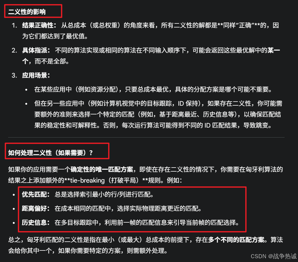
2.3 匈牙利匹配的二义性
匈牙利匹配(Hungarian Matching)在解决指派问题(Assignment Problem)时,其二义性(Ambiguity)指的是当存在多于一种方式可以达到相同的最优总成本(或总权重)时,算法可能返回不同的匹配方案。
简单来说,就是有不止一种“最佳答案”,他们在总分数上一样好,但具体的配对方式不同。
首先,快速回顾一下匈牙利算法:他是一种用于解决二分图的最小成本完美匹配问题(或最大权重完美匹配问题)的算法。
问题背景:假设你有N个人和N个任务,每个人完成每个任务都有一个特定的成本(或价值)。目标是为每个人分配一个任务(且每个任务只分配给一个人),使得总成本最小(或总价值最大)。
核心:算法会找到一个唯一的最优总成本。
匈牙利匹配的二义性示例
二义性不是指最优总成本不唯一,而是指达到这个最优总成本的匹配方案(即那些人匹配哪些任务)可能不唯一。
考虑一个简单的2*2的成本矩阵:
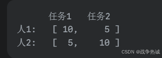
比如这种情况:
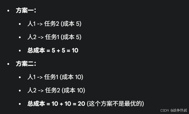
现在考虑另一种情况:
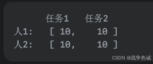
在这种情况下:
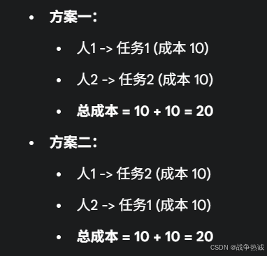
在这个例子中,总成本 20 是唯一的最小成本,但达到这个最小成本的匹配方案却有两种。这就是匈牙利匹配的二义性。当算法运行时,它可能会返回其中任意一个达到最优总成本的匹配方案。
为什么会出现二义性?
二义性通常发生在成本矩阵中存在对称性或多个零点排列方式时,在匈牙利算法的内部步骤中,当寻找独立的零点覆盖时,如果一个零点可以通过多条路径或选择来覆盖,并且这些不同的选择最终都导向相同的最优总成本,那么就会出现二义性。