当前位置：首页 > news >正文

机器学习 | 非线性回归拟合数据时的离群值检测

news 2025/7/6 0:55:30

非线性回归是一种用于模拟变量之间复杂关系的强大工具。然而，离群值的存在可能会显着扭曲结果，导致参数估计不准确和预测不可靠。因此，检测离群值对于稳健的非线性回归分析至关重要。本文深入研究了在非线性回归中识别离群值的方法和技术，确保您获得可靠和准确的结果。

了解非线性回归

什么是非线性回归？

非线性回归是回归分析的一种形式，其中观测数据由模型参数的非线性组合函数建模，并取决于一个或多个自变量。与线性回归不同，它假设变量之间的直线关系，非线性回归可以模拟更复杂的关系。

离群值检测的重要性
离群值是指显著偏离数据总体模式的数据点。在非线性回归的背景下，离群值可能对模型产生不成比例的影响，导致有偏的参数估计和较差的预测性能。检测和适当处理离群值对于保持回归分析的完整性至关重要。

非线性回归中离群值的检测方法

1.目视检查

散点图：散点图是直观检查数据是否存在潜在离群值的简单而有效的方法。通过绘制因变量与自变量的关系图，您可以确定与预期关系相差甚远的点。
残差图：残差图显示相对于自变量或拟合值的残差（观测值和预测值之间的差异）。离群值通常表现为具有较大残差的点，这些点与其余数据显著偏离。

2.统计方法

学生化残差：学生化残差是残差除以其标准差的估计值。它们遵循t分布，从而更容易识别离群值。具有大于特定阈值的学生化残差的点（例如，2或3）被认为是离群值。
Cook距离：Cook距离测量每个数据点对拟合值的影响。Cook距离大于特定阈值（通常为4/n，其中n为数据点数量）的点被视为有影响力和潜在离群值。
Hadi’s Potential：Hadi’s Potential是一种结合杠杆和残差来识别影响点的度量。它在非线性回归中特别有用，其中单独的杠杆可能不足以检测离群值。

3.鲁棒回归方法

最小绝对偏差（LAD）：最小绝对偏差最小化绝对残差之和，而不是残差平方之和。该方法对离群值不太敏感，并提供了普通最小二乘（OLS）回归的稳健替代方案。
M-估计：M-估计通过使用减少离群值影响的损失函数来推广最大似然估计。常用的M估计量包括Huber’s T和Tukey’s Bigweight。
最小二乘（LTS）：最小二乘回归最小化最小平方残差的总和，有效地忽略了可能由于离群值引起的最大残差。该方法在存在离群值的情况下提供稳健的参数估计。

非线性回归检测离群值：实例

步骤1：导入相关模块库

import numpy as np
import pandas as pd
import statsmodels.api as sm
import statsmodels.formula.api as smf
import matplotlib.pyplot as plt
import seaborn as sns
from statsmodels.robust.robust_linear_model import RLM
from statsmodels.robust.norms import HuberT, LeastSquares
from sklearn.metrics import mean_squared_error

步骤2：创建随机数据集

n = 100
x = np.linspace(0, 10, n)
y = 2.5 * np.sin(1.5 * x) + np.random.normal(0, 0.5, n)
# Adding some outliers
x_outliers = np.append(x, [1, 2, 3])
y_outliers = np.append(y, [10, -10, 12])
data = pd.DataFrame({'tumor_size': x_outliers, 'metastasis_fraction': y_outliers})

步骤3：使用普通最小二乘回归拟合非线性模型

# Adding a nonlinear term for the regression model
data['tumor_size_squared'] = data['tumor_size'] ** 2
ols_model = smf.ols('metastasis_fraction ~ tumor_size + tumor_size_squared', data=data).fit()

步骤4：可视化数据

plt.figure(figsize=(12, 6))
plt.subplot(1, 2, 1)
sns.scatterplot(x='tumor_size', y='metastasis_fraction', data=data)
plt.plot(data['tumor_size'], ols_model.fittedvalues, color='red')
plt.title('Scatter Plot with OLS Fit')plt.subplot(1, 2, 2)
sns.residplot(x=ols_model.fittedvalues, y=ols_model.resid)
plt.title('Residual Plot')
plt.show()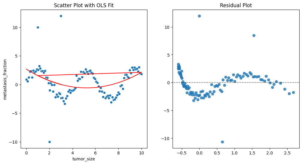

在这里插入图片描述

步骤5：应用于回归模型

# Robust regression using Least Absolute Deviations (LAD)
lad_model = smf.quantreg('metastasis_fraction ~ tumor_size + tumor_size_squared', data=data).fit(q=0.5)# Robust regression using M-Estimation with HuberT norm
rlm_huber = RLM(data['metastasis_fraction'], sm.add_constant(data[['tumor_size', 'tumor_size_squared']]), M=HuberT()).fit()

步骤6：使用统计方法识别离群值

# Studentized Residuals
data['studentized_residuals'] = ols_model.get_influence().resid_studentized_internal# Cook's Distance
data['cooks_distance'] = ols_model.get_influence().cooks_distance[0]# Hadi's Potential (not directly available in statsmodels, so we use an approximation)
data['leverage'] = ols_model.get_influence().hat_matrix_diag# Mark potential outliers
outlier_indices = data[(np.abs(data['studentized_residuals']) > 2) | (data['cooks_distance'] > 4/(n-2)) | (data['leverage'] > 0.2)].index
outliers = data.loc[outlier_indices]

步骤7：比较不同方法的结果

# OLS model
print("OLS Model Summary:")
print(ols_model.summary())# LAD model
print("\nLAD Model Summary:")
print(lad_model.summary())# RLM model with HuberT norm
print("\nRLM Model (HuberT) Summary:")
print(rlm_huber.summary())# Goodness-of-fit measures
print("\nGoodness-of-Fit Measures:")
print(f"OLS Mean Squared Error: {mean_squared_error(data['metastasis_fraction'], ols_model.fittedvalues)}")
print(f"LAD Mean Squared Error: {mean_squared_error(data['metastasis_fraction'], lad_model.fittedvalues)}")
print(f"RLM (HuberT) Mean Squared Error: {mean_squared_error(data['metastasis_fraction'], rlm_huber.fittedvalues)}")# Plotting the outliers
plt.figure(figsize=(12, 6))
sns.scatterplot(x='tumor_size', y='metastasis_fraction', data=data)
sns.scatterplot(x='tumor_size', y='metastasis_fraction', data=outliers, color='red')
plt.title('Scatter Plot with Outliers Highlighted')
plt.show()

输出

OLS Model Summary:OLS Regression Results                            
===============================================================================
Dep. Variable:     metastasis_fraction   R-squared:                       0.125
Model:                             OLS   Adj. R-squared:                  0.107
Method:                  Least Squares   F-statistic:                     7.134
Date:                 Tue, 30 Jul 2024   Prob (F-statistic):            0.00127
Time:                         21:15:45   Log-Likelihood:                -237.57
No. Observations:                  103   AIC:                             481.1
Df Residuals:                      100   BIC:                             489.0
Df Model:                            2                                         
Covariance Type:             nonrobust                                         
======================================================================================coef    std err          t      P>|t|      [0.025      0.975]
--------------------------------------------------------------------------------------
Intercept              2.6754      0.709      3.772      0.000       1.268       4.083
tumor_size            -1.2510      0.332     -3.769      0.000      -1.910      -0.593
tumor_size_squared     0.1196      0.032      3.712      0.000       0.056       0.183
==============================================================================
Omnibus:                       35.806   Durbin-Watson:                   1.658
Prob(Omnibus):                  0.000   Jarque-Bera (JB):              299.629
Skew:                           0.732   Prob(JB):                     8.64e-66
Kurtosis:                      11.226   Cond. No.                         142.
==============================================================================Notes:
[1] Standard Errors assume that the covariance matrix of the errors is correctly specified.LAD Model Summary:QuantReg Regression Results                          
===============================================================================
Dep. Variable:     metastasis_fraction   Pseudo R-squared:               0.1515
Model:                        QuantReg   Bandwidth:                       2.178
Method:                  Least Squares   Sparsity:                        5.458
Date:                 Tue, 30 Jul 2024   No. Observations:                  103
Time:                         21:15:45   Df Residuals:                      100Df Model:                            2
======================================================================================coef    std err          t      P>|t|      [0.025      0.975]
--------------------------------------------------------------------------------------
Intercept              3.0050      0.785      3.828      0.000       1.447       4.563
tumor_size            -1.6699      0.367     -4.545      0.000      -2.399      -0.941
tumor_size_squared     0.1686      0.036      4.729      0.000       0.098       0.239
======================================================================================RLM Model (HuberT) Summary:Robust linear Model Regression Results                    
===============================================================================
Dep. Variable:     metastasis_fraction   No. Observations:                  103
Model:                             RLM   Df Residuals:                      100
Method:                           IRLS   Df Model:                            2
Norm:                           HuberT                                         
Scale Est.:                        mad                                         
Cov Type:                           H1                                         
Date:                 Tue, 30 Jul 2024                                         
Time:                         21:15:45                                         
No. Iterations:                     11                                         
======================================================================================coef    std err          z      P>|z|      [0.025      0.975]
--------------------------------------------------------------------------------------
const                  2.5250      0.540      4.674      0.000       1.466       3.584
tumor_size            -1.2436      0.253     -4.919      0.000      -1.739      -0.748
tumor_size_squared     0.1208      0.025      4.923      0.000       0.073       0.169
======================================================================================If the model instance has been used for another fit with different fit parameters, then the fit options might not be the correct ones anymore .Goodness-of-Fit Measures:
OLS Mean Squared Error: 5.900980188225848
LAD Mean Squared Error: 6.09596526991115
RLM (HuberT) Mean Squared Error: 5.909805102901932