【超详图文】多少样本量用 t分布 OR 正态分布
文章目录
- 相关教程
- 相关文献
- 预备知识
- Lindeberg-Lévy中心极限定理
- t分布的来历
- 实验
- 不同分布不同抽样次数的总体分布
- 不同自由度相同参数的t分布&正态分布
作者:小猪快跑
基础数学&计算数学,从事优化领域7年+,主要研究方向:MIP求解器、整数规划、随机规划、智能优化算法
选择使用t分布还是正态分布通常取决于样本量的大小以及是否知道总体的标准差。
-
正态分布:
- 当样本量较大(通常n > 30)时,根据中心极限定理,无论原始总体分布是什么形状,样本均值的分布将接近正态分布。
- 如果总体标准差已知,并且你对总体均值进行推断,也可以使用正态分布,即使样本量较小。
-
t分布:
- 当样本量较小(n ≤ 30),并且总体标准差未知时,应该使用t分布。t分布与正态分布相似,但具有更宽的尾部,以反映小样本时更大的不确定性。
- t分布依赖于自由度的概念,自由度等于样本量减一(df = n - 1)。随着样本量增加,t分布逐渐逼近正态分布。
总结来说,如果你有一个小样本,并且不知道总体标准差,那么你应该使用t分布来进行统计推断。如果你有一个大样本,或者你知道总体标准差,那么你可以使用正态分布。在实际应用中,如果样本量足够大,两种分布之间的差异变得很小,这时可以认为两者是等价的。
如有错误,欢迎指正。如有更好的算法,也欢迎交流!!!——@小猪快跑
相关教程
- 常用分布的数学期望、方差、特征函数
- 【推导过程】常用离散分布的数学期望、方差、特征函数
- 【推导过程】常用连续分布的数学期望、方差、特征函数
- Z分位数速查表
- 【概率统计通俗版】极大似然估计
- 【超详图文】多少样本量用 t分布 OR 正态分布
- 【机器学习】【通俗版】EM算法(待更新)
相关文献
- [1] 茆诗松,周纪芗.概率论与数理统计 (第二版)[M].中国统计出版社,2000.
- [2] Bessel’s correction - Wikipedia
- [3] The t-distribution: a key statistical concept discovered by a beer brewery
- [4] Student’s t distribution | A Blog on Probability and Statistics
- [5] Student’s t distribution | Properties, proofs, exercises
预备知识
Lindeberg-Lévy中心极限定理
设 $ { X_n } $ 是独立同分布的随机变量序列, 且 $ E (X_n) = \mu $, $\mathrm{Var} (X_n)= \sigma^2 > 0 $.
记
Y n ∗ = X 1 + X 2 + ⋯ + X n − n μ σ n Y_n^* = \frac{X_1 + X_2 + \dotsb + X_n - n \mu}{\sigma \sqrt{n}} Yn∗=σnX1+X2+⋯+Xn−nμ
则对任意实数 $ y $, 有
lim n → + ∞ P ( Y n ∗ ≤ y ) = Φ ( y ) = 1 2 π ∫ − ∞ y e − t 2 / 2 d t . \lim_{n \to +\infty} P ( Y_n ^* \leq y ) = \Phi (y) = \frac{1}{\sqrt{2\pi}} \int_{-\infty}^y \mathrm{e}^{-t^2/2} \mathrm{d} t. n→+∞limP(Yn∗≤y)=Φ(y)=2π1∫−∞ye−t2/2dt.
t分布的来历
设 $ { X_n } $ 是独立同分布的随机变量序列, 且 $ E (X_n) = \mu $, $\mathrm{Var} (X_n)= \sigma^2 > 0 $
根据中心极限定理,我们知道
x ˉ − μ σ / n ∼ N ( 0 , 1 ) \frac{\bar{x}-\mu}{\sigma/\sqrt{n}} \sim N(0,1) σ/nxˉ−μ∼N(0,1)
但如果我们只有一些样本数据,其实无法知道准确的均值和方差,这时候就需要估计均值和方差。
我们来看一个例子。
设 $ { X_n } $ 是独立同分布的随机变量序列,且 $ \mu = 2500 $。抽样结果: 2051 , 2053 , 2055 , 2050 , 2051 2051,2053,2055,2050,2051 2051,2053,2055,2050,2051。则样本均值: 2052 2052 2052。
假如我们知道真实均值 $ \mu = 2500 $,则方差估计:
1 5 [ ( 2051 − 2050 ) 2 + ( 2053 − 2050 ) 2 + ( 2055 − 2050 ) 2 + ( 2050 − 2050 ) 2 + ( 2051 − 2050 ) 2 ] = 7.2 \frac{1}{5}[(2051-2050)^{2}+(2053-2050)^{2}+(2055-2050)^{2}+(2050-2050)^{2}+(2051-2050)^{2}]=7.2 51[(2051−2050)2+(2053−2050)2+(2055−2050)2+(2050−2050)2+(2051−2050)2]=7.2
假如我们使用样本均值 $ \mu = 2502 $,则方差估计:
1 5 [ ( 2051 − 2052 ) 2 + ( 2053 − 2052 ) 2 + ( 2055 − 2052 ) 2 + ( 2050 − 2052 ) 2 + ( 2051 − 2052 ) 2 ] = 3.2 \frac15[(2051-2052)^2+(2053-2052)^2+(2055-2052)^2+(2050-2052)^2+(2051-2052)^2]=3.2 51[(2051−2052)2+(2053−2052)2+(2055−2052)2+(2050−2052)2+(2051−2052)2]=3.2
我们发现样本均值计算的方差 << 实际均值计算的方差,下面我们将通过一个简单的数学恒等式 ( a + b ) 2 = a 2 + 2 a b + b 2 (a+b)^2=a^2+2ab+b^2 (a+b)2=a2+2ab+b2 证明
( 2053 − 2050 ⏟ 样本值与总体均值的偏差 ) 2 = [ ( 2053 − 2052 ⏟ 样本值与样本均值的偏差 ) ⏞ This is a . + ( 2052 − 2050 ⏟ 样本均值与总体均值的偏差 ) ⏞ This is b . ] 2 = ( 2053 − 2052 ) 2 ⏞ This is a 2 . + 2 ( 2053 − 2052 ) ( 2052 − 2050 ) ⏞ This is 2 a b . + ( 2052 − 2050 ) 2 ⏞ This is b 2 . \begin{aligned} (\underbrace{ \begin{array} {c}2053-2050 \end{array}}_{\text{样本值与总体均值的偏差}})^2 & =[\overbrace{(\underbrace{ \begin{array} {c}2053-2052 \end{array}}_{\text{样本值与样本均值的偏差}})}^{\text{This is }a.}+ \overbrace{(\underbrace{ \begin{array} {c}2052-2050 \end{array}}_{\text{样本均值与总体均值的偏差}})}^{\text{This is }b.}]^2 \\ & =\overbrace{\left(2053-2052\right)^2}^{\text{This is }a^2.}+\overbrace{2(2053-2052)(2052-2050)}^{\text{This is }2ab.}+\overbrace{\left(2052-2050\right)^2}^{\text{This is }b^2.} \end{aligned} (样本值与总体均值的偏差 2053−2050)2=[(样本值与样本均值的偏差 2053−2052) This is a.+(样本均值与总体均值的偏差 2052−2050) This is b.]2=(2053−2052)2 This is a2.+2(2053−2052)(2052−2050) This is 2ab.+(2052−2050)2 This is b2.
运用上面的公式,我们有
( 2051 − 2052 ) 2 ⏞ This is a 2 . + 2 ( 2051 − 2052 ) ( 2052 − 2050 ) ⏞ This is 2 a b . + ( 2052 − 2050 ) 2 ⏞ This is b 2 . ( 2053 − 2052 ) 2 + 2 ( 2053 − 2052 ) ( 2052 − 2050 ) + ( 2052 − 2050 ) 2 ( 2055 − 2052 ) 2 + 2 ( 2055 − 2052 ) ( 2052 − 2050 ) + ( 2052 − 2050 ) 2 ( 2050 − 2052 ) 2 + 2 ( 2050 − 2052 ) ( 2052 − 2050 ) + ( 2052 − 2050 ) 2 ( 2051 − 2052 ) 2 + 2 ( 2051 − 2052 ) ( 2052 − 2050 ) ⏟ 求和=0 + ( 2052 − 2050 ) 2 \overbrace{(2051-2052)^{2}}^{\text{This is }a^{2}.}+\overbrace{2(2051-2052)(2052-2050)}^{\text{This is }2ab.}+\overbrace{(2052-2050)^{2}}^{\text{This is }b^{2}.}\\ (2053-2052)^{2}+2(2053-2052)(2052-2050)+(2052-2050)^{2}\\ (2055-2052)^{2}+2(2055-2052)(2052-2050)+(2052-2050)^{2}\\ (2050-2052)^{2}+2(2050-2052)(2052-2050)+(2052-2050)^{2}\\ (2051-2052)^{2}+\underbrace{2(2051-2052)(2052-2050)}_{\text{求和=0}}+(2052-2050)^{2} (2051−2052)2 This is a2.+2(2051−2052)(2052−2050) This is 2ab.+(2052−2050)2 This is b2.(2053−2052)2+2(2053−2052)(2052−2050)+(2052−2050)2(2055−2052)2+2(2055−2052)(2052−2050)+(2052−2050)2(2050−2052)2+2(2050−2052)(2052−2050)+(2052−2050)2(2051−2052)2+求和=0 2(2051−2052)(2052−2050)+(2052−2050)2
实际均值计算的方差 a 2 + b 2 n \frac{a^2+b^2}n na2+b2 >= 样本均值计算的方差 a 2 n \frac{a^2}n na2
从例子中,我们知道样本均值计算的方差偏小,那我们现在来计算他的期望:
x ˉ = 1 n ∑ i = 1 n x i \bar{x}=\frac{1}{n}\sum_{i=1}^nx_i xˉ=n1i=1∑nxi
E [ 1 n ∑ k = 1 n ( x k − x ‾ ) 2 ] = n − 1 n ( E [ X 2 ] − E [ X ] 2 ) = n − 1 n V a r ( X ) \mathbb{E}\left[\frac{1}{n}\sum_{k=1}^n(x_k-\overline{x})^2\right]=\frac{n-1}{n}\left(\mathbb{E}[X^2]-\mathbb{E}[X]^2\right) = \frac{n-1}{n}\mathrm{Var}(X) E[n1k=1∑n(xk−x)2]=nn−1(E[X2]−E[X]2)=nn−1Var(X)
于是很自然的我们得到了无偏样本方差:
s 2 = 1 n − 1 ∑ i = 1 n ( x i − x ‾ ) 2 s^2=\frac{1}{n-1}\sum_{i=1}^n\left(x_i-\overline{x}\right)^2 s2=n−11i=1∑n(xi−x)2
那我们代入到之前的公式:
x ˉ − μ s / n ∼ t ( n − 1 ) \frac{\bar{x}-\mu}{s/\sqrt{n}} \sim t(n-1) s/nxˉ−μ∼t(n−1)
就会呈现一个自由度为 n − 1 n-1 n−1 的 T T T 分布,其中 n n n 是样本的数量。
注: s s s 的计算过程中依赖 ( x i − x ˉ ) (x_{i}-\bar{x}) (xi−xˉ) 的值,而这就产生了一个隐藏的限制, ∑ i = 1 n ( x i − x ) = 0 \sum_{i=1}^{n}(x_{i}-x)=0 ∑i=1n(xi−x)=0。所以这使得一旦前 n − 1 n-1 n−1 个 ( x i − x ˉ ) (x_{i}-\bar{x}) (xi−xˉ) 确定后,第 n n n 个 ( x i − x ˉ ) (x_{i}-\bar{x}) (xi−xˉ) 立马被锁定。自由度因此变成了 n − 1 n-1 n−1。
实验
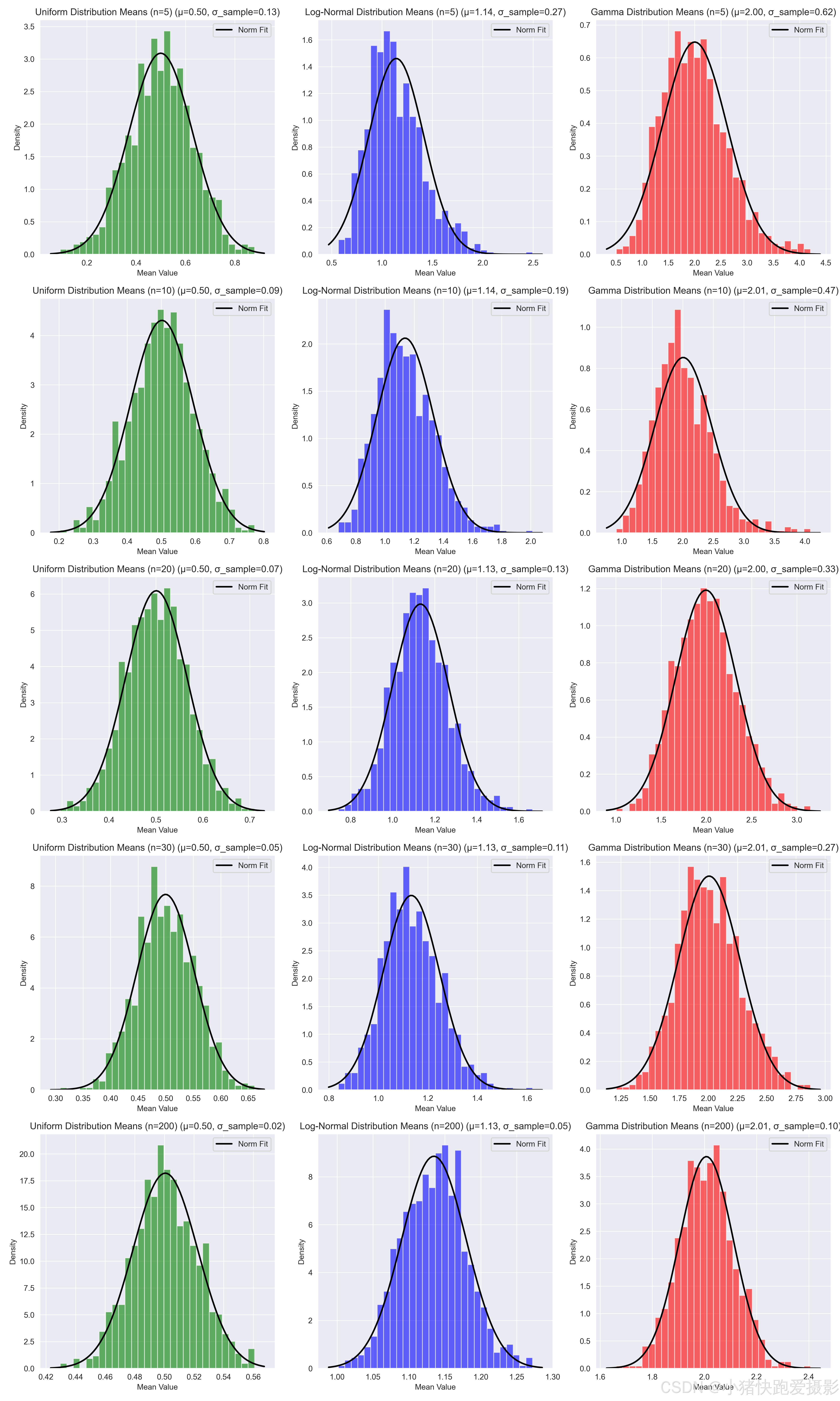
不同分布不同抽样次数的总体分布
import numpy as np
import matplotlib.pyplot as plt
from scipy.stats import lognorm, gamma, norm, t# 设置重复次数
repeats = 1000    # 重复抽取样本的次数# 定义分布参数
uniform_low, uniform_high = 0, 1
lognorm_s = 0.5  # 对数正态分布形状参数
gamma_shape = 2  # 伽玛分布形状参数# 定义要测试的样本量
sample_sizes = [5, 10, 20, 30, 200]# 函数:绘制直方图和正态及t分布拟合曲线
def plot_distribution_with_fits(data, ax, color='b', title=''):# 计算样本均值和样本标准差mu = np.mean(data)std_sample = np.std(data, ddof=1)  # 使用ddof=1来获得无偏样本标准差# 绘制直方图ax.hist(data, bins=30, density=True, alpha=0.6, color=color)# 绘制正态拟合曲线xmin, xmax = ax.get_xlim()x = np.linspace(xmin, xmax, 100)p_norm = norm.pdf(x, mu, std_sample)ax.plot(x, p_norm, 'k', linewidth=2, label='Norm Fit')title += f' (μ={mu:.2f}, σ_sample={std_sample:.2f})'ax.set_title(title)ax.set_xlabel('Mean Value')ax.set_ylabel('Density')ax.legend()# 创建子图并绘制图形
fig, axes = plt.subplots(len(sample_sizes), 3, figsize=(15, 25))for i, sample_size in enumerate(sample_sizes):# 初始化存储均值的列表means_uniform = []means_lognorm = []means_gamma = []# 抽取样本并计算均值for _ in range(repeats):# 均匀分布sample_uniform = np.random.uniform(uniform_low, uniform_high, sample_size)means_uniform.append(np.mean(sample_uniform))# 对数正态分布sample_lognorm = lognorm.rvs(s=lognorm_s, size=sample_size)means_lognorm.append(np.mean(sample_lognorm))# 伽玛分布sample_gamma = gamma.rvs(a=gamma_shape, size=sample_size)means_gamma.append(np.mean(sample_gamma))# 应用到每个分布plot_distribution_with_fits(means_uniform, axes[i, 0], color='g', title=f'Uniform Distribution Means (n={sample_size})')plot_distribution_with_fits(means_lognorm, axes[i, 1], color='b', title=f'Log-Normal Distribution Means (n={sample_size})')plot_distribution_with_fits(means_gamma, axes[i, 2], color='r', title=f'Gamma Distribution Means (n={sample_size})')# 展示图形
plt.tight_layout()
plt.savefig('figures/Distribution Means.png', dpi=300)
plt.show()
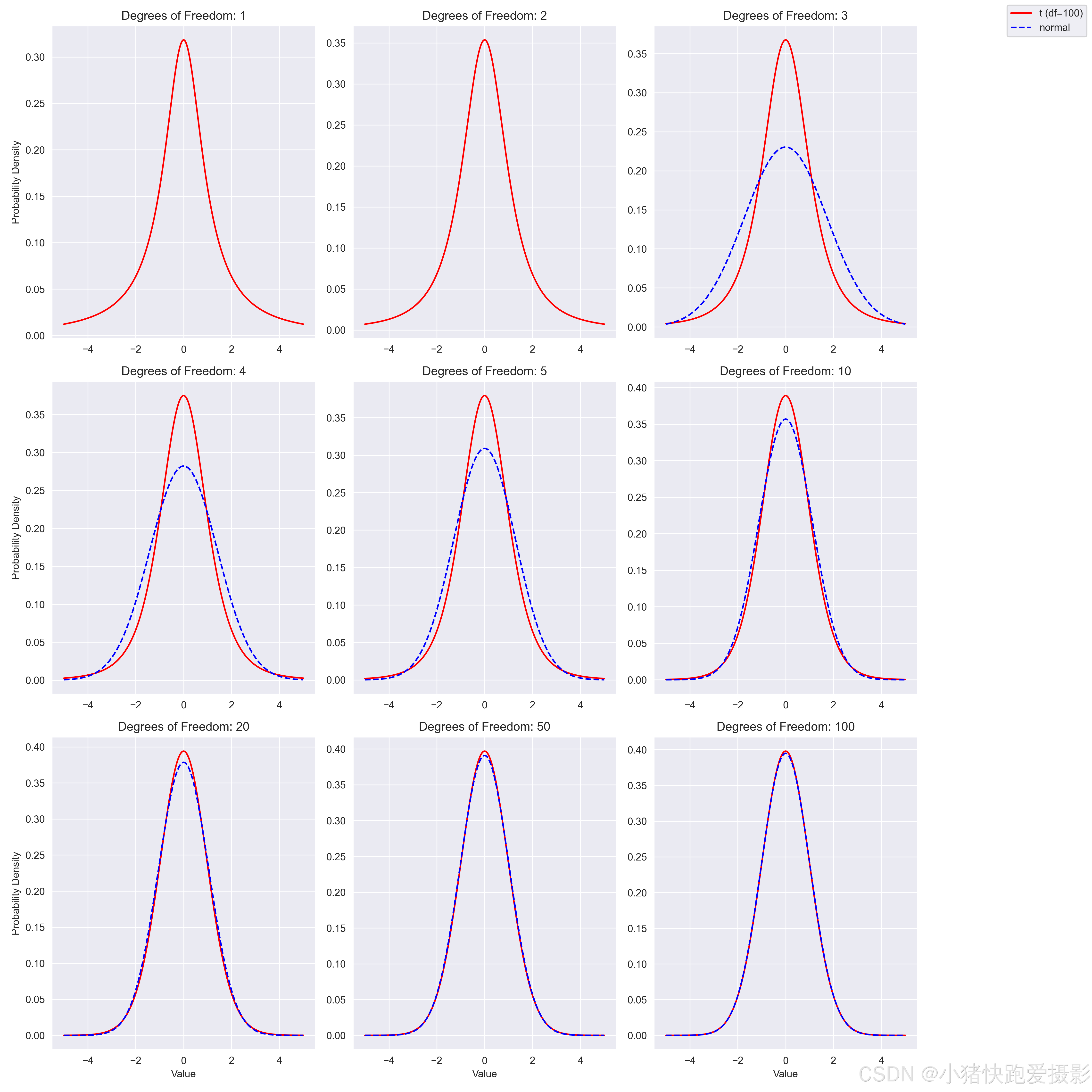
不同自由度相同参数的t分布&正态分布
import numpy as np
import matplotlib.pyplot as plt
from scipy.stats import t, norm# 定义x轴的范围
x = np.linspace(-5, 5, 1000)# 定义要比较的t分布的不同自由度df列表
dfs = [1, 2, 3, 4, 5, 10, 20, 50, 100]# 创建一个3x3的子图网格
fig, axs = plt.subplots(3, 3, figsize=(15, 15))# 遍历不同的自由度并绘制对应的t分布和正态分布
for ax, df in zip(axs.flat, dfs):# 计算t分布的概率密度函数t_pdf = t.pdf(x, df)# 假设正态分布具有与t分布相同的均值(0)和标准差(sqrt(df/(df-2)),当df>2时)normal_pdf = norm.pdf(x, loc=0, scale=np.sqrt(df / (df - 2))) if df > 2 else None# 绘制t分布ax.plot(x, t_pdf, label=f't (df={df})', linestyle='-', color='red')# 如果df允许,绘制正态分布if normal_pdf is not None:ax.plot(x, normal_pdf, label='normal', linestyle='--', color='blue')# 添加标题ax.set_title(f'Degrees of Freedom: {df}')ax.grid(True)# 只在最下面一行添加xlabel,在最左边一列添加ylabel以保持整洁if ax.get_subplotspec().is_last_row():ax.set_xlabel('Value')if ax.get_subplotspec().is_first_col():ax.set_ylabel('Probability Density')# 添加一个总的图例到图表中
handles, labels = ax.get_legend_handles_labels()
fig.legend(handles, labels, loc='upper right')# 调整布局以防止重叠
plt.tight_layout(rect=[0, 0, 0.85, 1])  # 为图例留出空间plt.savefig('figures/t VS normal Distribution.png', dpi=300)# 显示图表
plt.show()