当前位置：首页 > news >正文

CNN神经网络——手写体识别

news 2025/8/28 5:13:18

Load The Datesets

Defining,Training,Measuring CNN Algorithm

Datasets

GRAET HONOR TO SHARE MY KNOWLEDGE WITH YOU

This paper is going to show how to use keras to relize a CNN model for digits classfication

Load The Datesets

The datasets files are shown in the follwing chart:

we see, there are all .gz file, which is a common zipped file format. And differ from some datasets needed to be splitted as training sest and testting set, this datasets shown above is already be splitted as traning and testing set, where file t10k-images-idx3-ubyte.gz and t10k-labels-idx1-ubyte.gz is the features and labels of testing sets respectively, while the other two is features and labels of traning sets. When upzipping those files, one could find there is a binary file:

As we see, this file is not CSV , XLSX, DATA or other image file like PNG, JPG or JPEG. So How to read it to Python is another problem we have to deal with. Since is not our focus, there I just show the code:

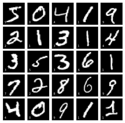
def data_generate():import gzipdatadir = r'..\数据集\MNIST_data'   #datadir为解压路径sources = ['t10k-images-idx3-ubyte.gz','t10k-labels-idx1-ubyte.gz','train-images-idx3-ubyte.gz','train-labels-idx1-ubyte.gz']"""函数说明：def extract_tar函数用于解压某个tar.gz的压缩文件。"""def extract_tar(datafile,extractdir):   #定义一个解压缩函数file = datafile.replace(".gz","")g_file = gzip.GzipFile(datafile)#读取解压后的文件，并写入去掉后缀名的同名文件（即得到解压后的文件）open(file, "wb+").write(g_file.read())    #将文件加压缩到压缩文件所在的文件夹中g_file.close()print("%s 解压完成."%datafile)return file   #返回解压缩后文件的名称字符串data_file = []    for source in sources:    #通过遍历解压文件夹datasets_q8中所有文件datafile = r'%s\%s' %(datadir,source)   #指定待解压缩文件file = extract_tar(datafile,datadir)    #将文件压缩到路径datadirdata_file.append(file)"""很多类型的文件，其起始的几个字节的内容是固定的(或是有意填充，或是本就如此)。根据这几个字节的内容就可以确定文件类型，因此这几个字节的内容被称为魔数 (magic number)。"""import structimport numpy as npdef decode_idx1_ubyte(idx1_ubyte_file):"""解析idx1文件的通用函数:param idx1_ubyte_file: idx1文件路径:return: 数据集"""# 读取二进制数据bin_data = open(idx1_ubyte_file, 'rb').read()# 解析文件头信息，依次为魔数和标签数offset = 0fmt_header = '>ii'magic_number, num_images = struct.unpack_from(fmt_header, bin_data, offset)print('魔数:%d, 图片数量: %d张' % (magic_number, num_images))# 解析数据集offset += struct.calcsize(fmt_header)fmt_image = '>B'labels = np.empty(num_images)for i in range(num_images):if (i + 1) % 10000 == 0:print ('已解析 %d' % (i + 1) + '张')labels[i] = struct.unpack_from(fmt_image, bin_data, offset)[0]offset += struct.calcsize(fmt_image)return labelsy_train = decode_idx1_ubyte(data_file[3])y_test = decode_idx1_ubyte(data_file[1])y_train = y_train.astype(np.int)y_test = y_test.astype(np.int)def decode_idx3_ubyte(idx3_ubyte_file):"""解析idx3文件的通用函数:param idx3_ubyte_file: idx3文件路径:return: 数据集"""# 读取二进制数据bin_data = open(idx3_ubyte_file, 'rb').read()# 解析文件头信息，依次为魔数、图片数量、每张图片高、每张图片宽offset = 0fmt_header = '>iiii' #因为数据结构中前4行的数据类型都是32位整型，所以采用i格式，但我们需要读取前4行数据，所以需要4个i。我们后面会看到标签集中，只使用2个ii。magic_number, num_images, num_rows, num_cols = struct.unpack_from(fmt_header, bin_data, offset)print('魔数:%d, 图片数量: %d张, 图片大小: %d*%d' % (magic_number, num_images, num_rows, num_cols))# 解析数据集image_size = num_rows * num_colsoffset += struct.calcsize(fmt_header)  #获得数据在缓存中的指针位置，从前面介绍的数据结构可以看出，读取了前4行之后，指针位置（即偏移位置offset）指向0016。print(offset)fmt_image = '>' + str(image_size) + 'B'  #图像数据像素值的类型为unsigned char型，对应的format格式为B。这里还有加上图像大小784，是为了读取784个B格式数据，如果没有则只会读取一个值（即一副图像中的一个像素值）print(fmt_image,offset,struct.calcsize(fmt_image))images = np.empty((num_images, num_rows, num_cols))#plt.figure()for i in range(num_images):if (i + 1) % 10000 == 0:print('已解析 %d' % (i + 1) + '张')print(offset)images[i] = np.array(struct.unpack_from(fmt_image, bin_data, offset)).reshape((num_rows, num_cols))offset += struct.calcsize(fmt_image)return imagesX_train = decode_idx3_ubyte(data_file[2])X_test = decode_idx3_ubyte(data_file[0])"""画图代码：读者可以运行该代码直观地查看数据集"""import matplotlib.pyplot as pltfig, axes = plt.subplots(5,5, figsize=(8, 8),subplot_kw={'xticks':[], 'yticks':[]},gridspec_kw=dict(hspace=0.1, wspace=0.1))for i, ax in enumerate(axes.flat):ax.imshow(X_train[i], cmap='gray', interpolation='nearest')ax.text(0.07, 0.07, str(y_train[i]),transform=ax.transAxes, color='white')return X_train,y_train,X_test,y_test

The above code define a function that generates the features of Trainingset denoted as X_train, labels of Trainingset denoted as y_train, and X_test, y_test of Testingset. Meanwhile, the above code plotting some of the datasets, shown below:

Defining,Training,Measuring CNN Algorithm

This section we will construct, traning a CNN model ,and measuring it in the testing sets using accuracy score

We run the function to gain dataset:

X_train,y_train,X_test,y_test = data_generate()

Then we import some useful package:

from keras.utils import to_categorical
from keras.models import Sequential
from keras.layers import Dense, Activation, Dropout, Conv2D,AveragePooling2D,Flatten

Then we define the CNN model :

model = Sequential()   #创建神经网络类
model.add(Conv2D(16,kernel_size=(3,3),input_shape=(width,height,1),activation='relu'))    #创建一个卷积层，核为3X3
model.add(Dropout(0.2))    #Dropout正则化
model.add(Conv2D(32,kernel_size=(3,3),activation='relu'))
model.add(Dropout(0.2))
model.add(AveragePooling2D(pool_size=(2,2)))    #添加池化层，并根据平均值将矩阵缩放成2X2
model.add(Dropout(0.2))
model.add(Conv2D(64,kernel_size=(3,3),activation='relu'))
model.add(AveragePooling2D(pool_size=(2,2)))    #添加池化层，缩放成2X2
model.add(Flatten())    #添加Flatten层
model.add(Dense(units=512,activation='relu'))    #BP神经网络的隐藏层，512个节点
model.add(Dense(units=10,activation='sigmoid'))    #输出层

For the principle of Convolution layer or Pooling layer, please refer to
https://blog.csdn.net/weixin_42141390/article/details/105004900

Then we select Adam as the algorithm to finding the parameters of the CNN model with cross-entropy as cost function，then we set the max iteration is 100, the code is shown as below:

model.compile(optimizer='adam',loss='binary_crossentropy',metrics=['accuracy'])    #使用Adam算法训练模型
history = model.fit(X_train,y_train,epochs=100,batch_size=256,validation_data=(X_test,y_test))    #定义随机搜索算法的mini-batch=256

Running the code, the output windows will show the following information:

Epoch 1/100

60000/60000 [==============================] - 219s 4ms/step - loss: 0.0869 - acc: 0.9712 - val_loss: 0.0199 - val_acc: 0.9934

..........

Epoch 99/100

60000/60000 [==============================] - 186s 3ms/step - loss: 2.6969e-05 - acc: 1.0000 - val_loss: 0.0109 - val_acc: 0.9986

Epoch 100/100

60000/60000 [==============================] - 186s 3ms/step - loss: 2.6969e-05 - acc: 1.0000 - val_loss: 0.0110 - val_acc: 0.9986

Then we plot the training curve by varible "history"，using the following code:

import matplotlib.pyplot as plt
font1 = {'family' : 'Times New Roman',
'weight' : 'normal',
'size'   : 20,
}
plt.rcParams['font.sans-serif']=['SimHei']
plt.rcParams['axes.unicode_minus'] = False
plt.plot(history.history['acc'],linewidth=3,label='Train')
plt.plot(history.history['val_acc'],linewidth=3,linestyle='dashed',label='Test')
plt.xlabel('Epoch',fontsize=20)
plt.ylabel('精确度',fontsize=20)
plt.legend(prop=font1)