Python综合数据分析_RFM用户分层模型
文章目录
- 1.数据加载
- 2.查看数据情况
- 3.数据合并及填充
- 4.查看特征字段之间相关性
- 5.聚合操作
- 6.时间维度上看销售额
- 7.计算用户RFM
- 8.数据保存存储
- (1).to_csv
- (1).to_pickle
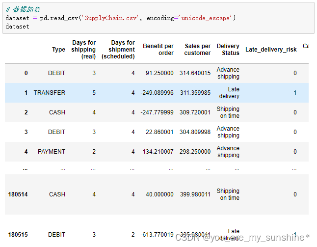
1.数据加载
import pandas as pd
dataset = pd.read_csv('SupplyChain.csv', encoding='unicode_escape')
dataset
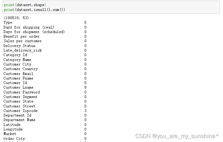
2.查看数据情况
print(dataset.shape)
print(dataset.isnull().sum())

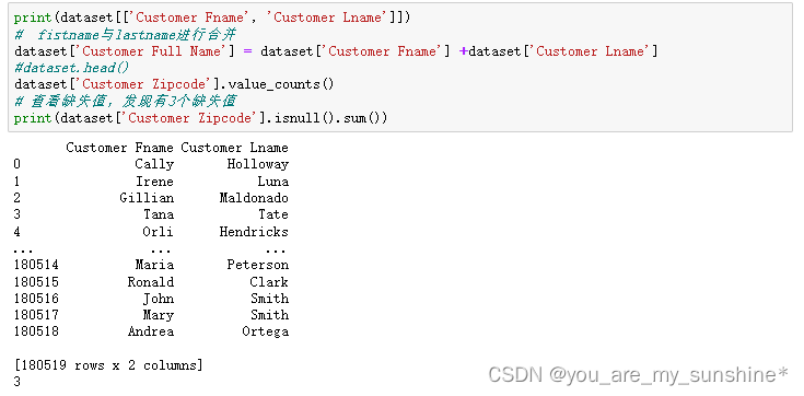
3.数据合并及填充
print(dataset[['Customer Fname', 'Customer Lname']])
#  fistname与lastname进行合并
dataset['Customer Full Name'] = dataset['Customer Fname'] +dataset['Customer Lname']
#dataset.head()
dataset['Customer Zipcode'].value_counts()
# 查看缺失值,发现有3个缺失值
print(dataset['Customer Zipcode'].isnull().sum())
dataset['Customer Zipcode'] = dataset['Customer Zipcode'].fillna(0)
dataset.head()

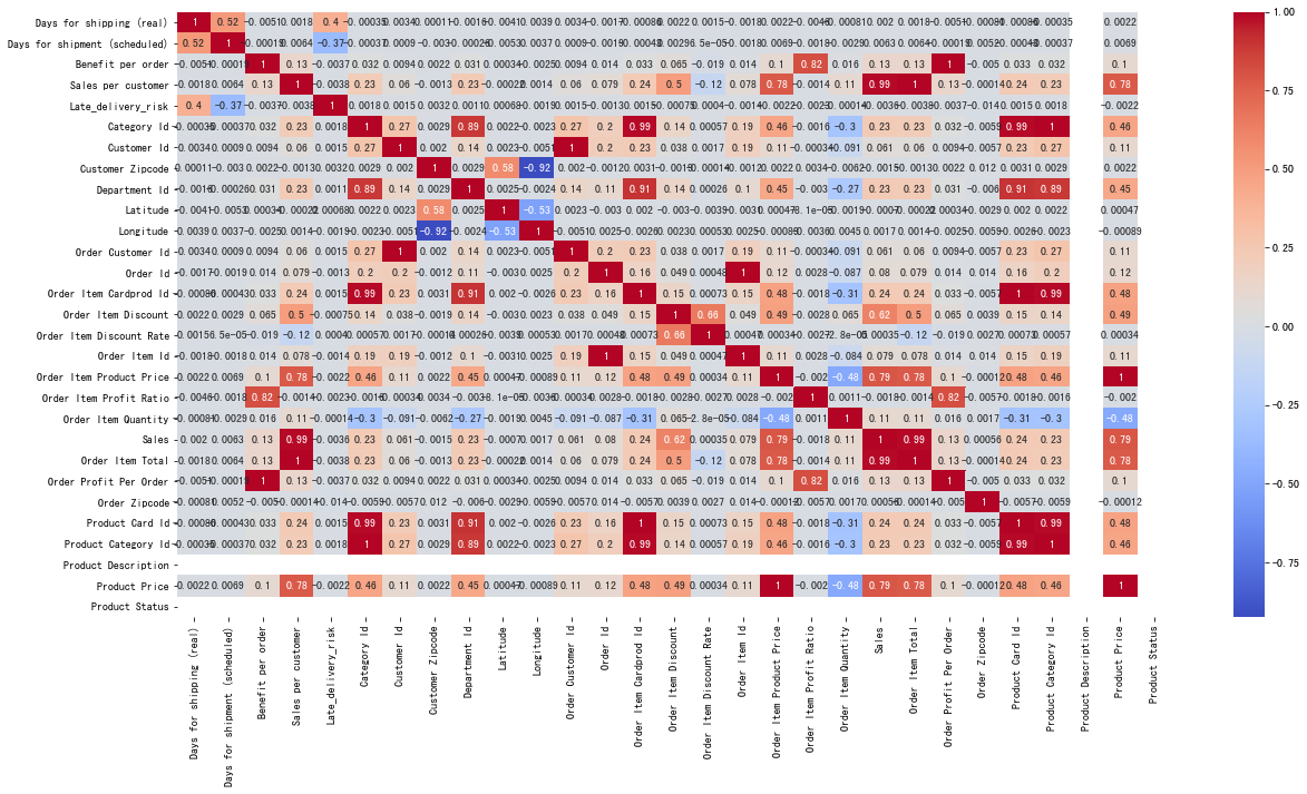
4.查看特征字段之间相关性
import matplotlib.pyplot as plt
import seaborn as sns
# 特征字段之间相关性 热力图
data = dataset
plt.figure(figsize=(20,10))
# annot=True 显示具体数字
sns.heatmap(data.corr(), annot=True, cmap='coolwarm')
# 结论:可以观察到Product Price和Sales,Order Item Total有很高的相关性
5.聚合操作
# 基于Market进行聚合
market = data.groupby('Market')
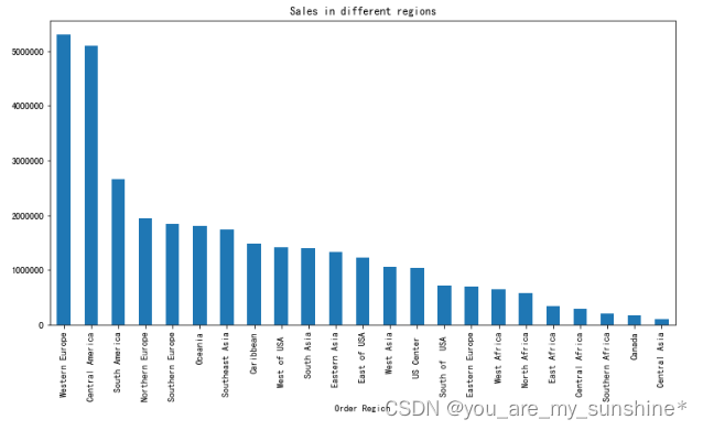
# 基于Region进行聚合
region = data.groupby('Order Region')
plt.figure(1)
market['Sales per customer'].sum().sort_values(ascending=False).plot.bar(figsize=(12,6), title='Sales in different markets')
plt.figure(2)
region['Sales per customer'].sum().sort_values(ascending=False).plot.bar(figsize=(12,6), title='Sales in different regions')
plt.show()

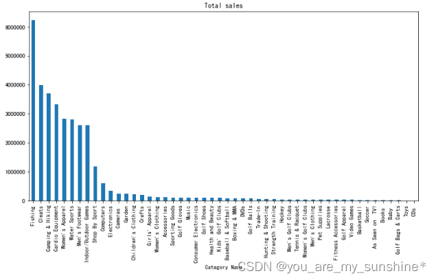
# 基于Category Name进行聚类
cat = data.groupby('Category Name')
plt.figure(1)
# 不同类别的 总销售额
cat['Sales per customer'].sum().sort_values(ascending=False).plot.bar(figsize=(12,6), title='Total sales')
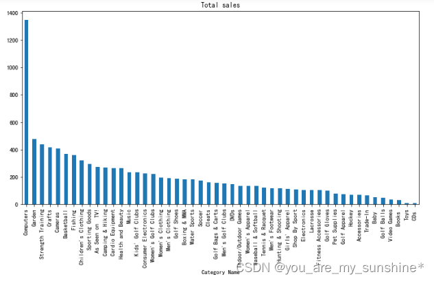
plt.figure(2)
# 不同类别的 平均销售额
cat['Sales per customer'].mean().sort_values(ascending=False).plot.bar(figsize=(12,6), title='Total sales')
plt.show()
6.时间维度上看销售额
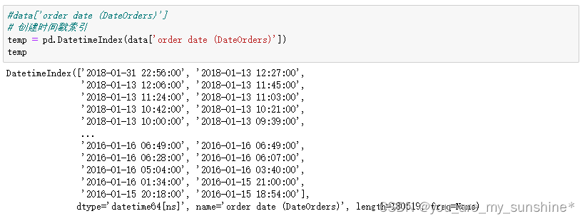
#data['order date (DateOrders)']
# 创建时间戳索引
temp = pd.DatetimeIndex(data['order date (DateOrders)'])
temp
# 取order date (DateOrders)字段中的year, month, weekday, hour, month_year
data['order_year'] = temp.year
data['order_month'] = temp.month
data['order_week_day'] = temp.weekday
data['order_hour'] = temp.hour
data['order_month_year'] = temp.to_period('M')
data.head()

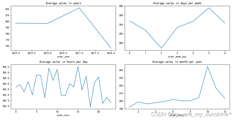
# 对销售额进行探索,按照不同时间维度 年,星期,小时,月
plt.figure(figsize=(10, 12))
plt.subplot(4, 2, 1)
df_year = data.groupby('order_year')
df_year['Sales'].mean().plot(figsize=(12, 12), title='Average sales in years')
plt.subplot(4, 2, 2)
df_day = data.groupby('order_week_day')
df_day['Sales'].mean().plot(figsize=(12, 12), title='Average sales in days per week')
plt.subplot(4, 2, 3)
df_hour = data.groupby('order_hour')
df_hour['Sales'].mean().plot(figsize=(12, 12), title='Average sales in hours per day')
plt.subplot(4, 2, 4)
df_month = data.groupby('order_month')
df_month['Sales'].mean().plot(figsize=(12, 12), title='Average sales in month per year')
plt.tight_layout()
plt.show()
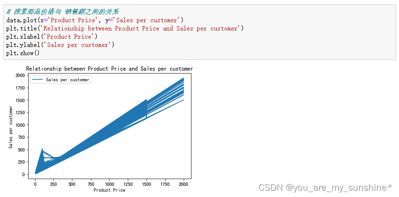
# 探索商品价格与 销售额之间的关系
data.plot(x='Product Price', y='Sales per customer')
plt.title('Relationship between Product Price and Sales per customer')
plt.xlabel('Product Price')
plt.ylabel('Sales per customer')
plt.show()
7.计算用户RFM
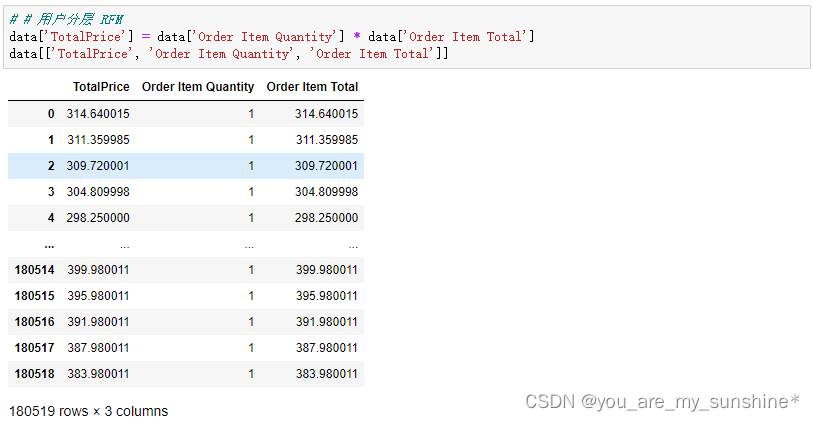
# # 用户分层 RFM
data['TotalPrice'] = data['Order Item Quantity'] * data['Order Item Total']
data[['TotalPrice', 'Order Item Quantity', 'Order Item Total']]
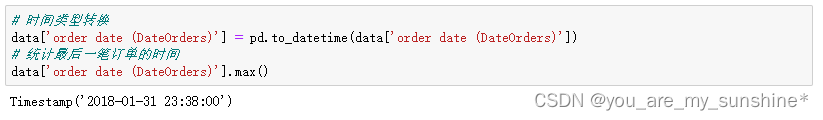
# 时间类型转换
data['order date (DateOrders)'] = pd.to_datetime(data['order date (DateOrders)'])
# 统计最后一笔订单的时间
data['order date (DateOrders)'].max()
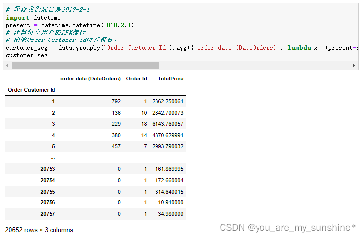
# 假设我们现在是2018-2-1
import datetime
present = datetime.datetime(2018,2,1)
# 计算每个用户的RFM指标
# 按照Order Customer Id进行聚合,
customer_seg = data.groupby('Order Customer Id').agg({'order date (DateOrders)': lambda x: (present-x.max()).days,                                                       'Order Id': lambda x:len(x), 'TotalPrice': lambda x: x.sum()})
customer_seg
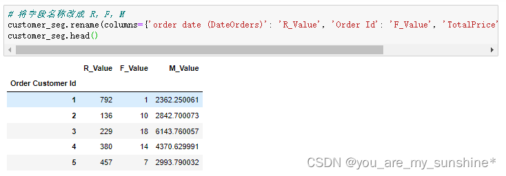
# 将字段名称改成 R,F,M
customer_seg.rename(columns={'order date (DateOrders)': 'R_Value', 'Order Id': 'F_Value', 'TotalPrice': 'M_Value'}, inplace=True)
customer_seg.head()
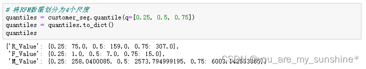
# 将RFM数据划分为4个尺度
quantiles = customer_seg.quantile(q=[0.25, 0.5, 0.75])
quantiles = quantiles.to_dict()
quantiles
# R_Value越小越好 => R_Score就越大
def R_Score(a, b, c):if a <= c[b][0.25]:return 4elif a <= c[b][0.50]:return 3elif a <= c[b][0.75]:return 2else:return 1# F_Value, M_Value越大越好
def FM_Score(a, b, c):if a <= c[b][0.25]:return 1elif a <= c[b][0.50]:return 2elif a <= c[b][0.75]:return 3else:return 4
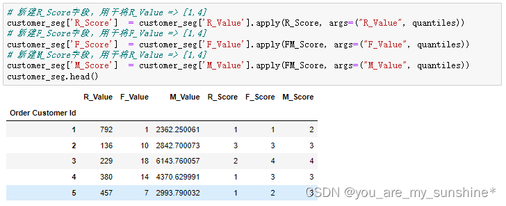
# 新建R_Score字段,用于将R_Value => [1,4]
customer_seg['R_Score']  = customer_seg['R_Value'].apply(R_Score, args=("R_Value", quantiles))
# 新建F_Score字段,用于将F_Value => [1,4]
customer_seg['F_Score']  = customer_seg['F_Value'].apply(FM_Score, args=("F_Value", quantiles))
# 新建M_Score字段,用于将R_Value => [1,4]
customer_seg['M_Score']  = customer_seg['M_Value'].apply(FM_Score, args=("M_Value", quantiles))
customer_seg.head()
# 计算RFM用户分层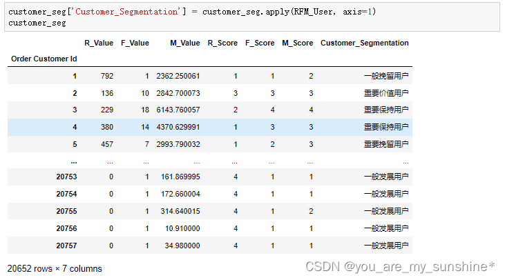
def RFM_User(df):if df['M_Score'] > 2 and df['F_Score'] > 2 and df['R_Score'] > 2:return '重要价值用户'if df['M_Score'] > 2 and df['F_Score'] <= 2 and df['R_Score'] > 2:return '重要发展用户'if df['M_Score'] > 2 and df['F_Score'] > 2 and df['R_Score'] <= 2:return '重要保持用户'if df['M_Score'] > 2 and df['F_Score'] <= 2 and df['R_Score'] <= 2:return '重要挽留用户'if df['M_Score'] <= 2 and df['F_Score'] > 2 and df['R_Score'] > 2:return '一般价值用户'if df['M_Score'] <= 2 and df['F_Score'] <= 2 and df['R_Score'] > 2:return '一般发展用户'if df['M_Score'] <= 2 and df['F_Score'] > 2 and df['R_Score'] <= 2:return '一般保持用户'if df['M_Score'] <= 2 and df['F_Score'] <= 2 and df['R_Score'] <= 2:return '一般挽留用户'customer_seg['Customer_Segmentation'] = customer_seg.apply(RFM_User, axis=1)
customer_seg
8.数据保存存储
(1).to_csv
customer_seg.to_csv('supply_chain_rfm_result.csv', index=False)
(1).to_pickle
# 数据预处理后,将处理后的数据进行保存
data.to_pickle('data.pkl')
参考资料:开课吧