当前位置：首页 > news >正文

CNN对 MNIST 数据库中的图像进行分类

news 2025/9/10 22:01:22

加载 MNIST 数据库

MNIST 是机器学习领域最著名的数据集之一。

它有 70,000 张手写数字图像 - 下载非常简单 - 图像尺寸为 28x28 - 灰度图

from keras.datasets import mnist# 使用 Keras 导入MNIST 数据库
(X_train, y_train), (X_test, y_test) = mnist.load_data()print("The MNIST database has a training set of %d examples." % len(X_train))
print("The MNIST database has a test set of %d examples." % len(X_test))

将前六个训练图像可视化

import matplotlib.pyplot as plt
%matplotlib inline
import matplotlib.cm as cm
import numpy as np# 绘制前六幅训练图像
fig = plt.figure(figsize=(20,20))
for i in range(6):ax = fig.add_subplot(1, 6, i+1, xticks=[], yticks=[])ax.imshow(X_train[i], cmap='gray')ax.set_title(str(y_train[i]))

查看图像的更多细节

def visualize_input(img, ax):ax.imshow(img, cmap='gray')width, height = img.shapethresh = img.max()/2.5for x in range(width):for y in range(height):ax.annotate(str(round(img[x][y],2)), xy=(y,x),horizontalalignment='center',verticalalignment='center',color='white' if img[x][y]<thresh else 'black')fig = plt.figure(figsize = (12,12)) 
ax = fig.add_subplot(111)
visualize_input(X_train[0], ax)

预处理输入图像：通过将每幅图像中的每个像素除以 255 来调整图像比例

# 调整比例，使数值在 0 - 1 范围内 [0,255] --> [0,1]
X_train = X_train.astype('float32')/255
X_test = X_test.astype('float32')/255 print('X_train shape:', X_train.shape)
print(X_train.shape[0], 'train samples')
print(X_test.shape[0], 'test samples')

对标签进行预处理：使用单热方案对分类整数标签进行编码

from keras.utils import to_categoricalnum_classes = 10 
# 打印前十个（整数值）训练标签
print('Integer-valued labels:')
print(y_train[:10])# 对标签进行一次性编码
# 将类别向量转换为二进制类别矩阵
y_train = to_categorical(y_train, num_classes)
y_test = to_categorical(y_test, num_classes)# 打印前十个（单次）训练标签
print('One-hot labels:')
print(y_train[:10])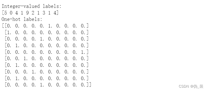

重塑数据以适应我们的 CNN（和 input_shape）

# 输入图像尺寸为 28x28 像素的图像。
img_rows, img_cols = 28, 28X_train = X_train.reshape(X_train.shape[0], img_rows, img_cols, 1)
X_test = X_test.reshape(X_test.shape[0], img_rows, img_cols, 1)
input_shape = (img_rows, img_cols, 1)print('input_shape: ', input_shape)
print('x_train shape:', X_train.shape)

定义模型架构

您必须传递以下参数：

filters - 滤波器的数量。
kernel_size - 指定（正方形）卷积窗口高度和宽度的数值。

还有一些额外的、可选的参数需要调整：

strides - 卷积的步长。如果不指定任何参数，strides 将设为 1。
padding - "有效 "或 "相同 "之一。如果不做任何指定，padding 将设置为 "有效"。
activation - 通常为 "relu"。如果不指定任何内容，则不会应用激活。我们强烈建议你为网络中的每个卷积层添加 ReLU 激活函数。

需要注意的事项

始终为 CNN 中的 Conv2D 层添加 ReLU 激活函数。除网络中的最后一层外，密集层也应具有 ReLU 激活函数。
在构建分类网络时，网络的最终层应是具有 softmax 激活函数的密集层。最终层的节点数应等于数据集中的类总数。

from keras.models import Sequential
from keras.layers import Conv2D, MaxPooling2D, Flatten, Dense, Dropout# 创建模型对象
model = Sequential()# CONV_1: 添加 CONV 层，采用 RELU 激活，深度 = 32 内核
model.add(Conv2D(32, kernel_size=(3, 3), padding='same',activation='relu',input_shape=(28,28,1)))
# POOL_1: 对图像进行下采样，选择最佳特征
model.add(MaxPooling2D(pool_size=(2, 2)))# CONV_2: 在这里，我们将深度增加到 64
model.add(Conv2D(64, (3, 3),padding='same', activation='relu'))
# POOL_2: more downsampling
model.add(MaxPooling2D(pool_size=(2, 2)))# 由于维度过多，我们只需要一个分类输出
model.add(Flatten())# FC_1: 完全连接，获取所有相关数据
model.add(Dense(64, activation='relu'))# FC_2: 输出软最大值，将矩阵压制成 10 个类别的输出概率
model.add(Dense(10, activation='softmax'))model.summary()

需要注意的事项：

网络以两个卷积层的序列开始，然后是最大池化层。
最后一层为数据集中的每个对象类别设置了一个条目，并具有软最大激活函数，因此可以返回概率。
Conv2D 深度从输入层的 1 增加到 32 到 64。
我们还想减少高度和宽度--这就是 maxpooling 的作用所在。请注意，在池化层之后，图像尺寸从 28 减小到 14。
可以看到，每个输出形状都用 None 代替了批量大小。这是为了便于在运行时更改批次大小。
最后，我们会添加一个或多个全连接层来确定图像中包含的对象。例如，如果在上一个最大池化层中发现了车轮，那么这个 FC 层将转换该信息，以更高的概率预测图像中出现了一辆汽车。如果图像中有眼睛、腿和尾巴，那么这可能意味着图像中有一只狗。

编译模型

# rmsprop 和自适应学习率 (adaDelta) 是梯度下降的流行形式，仅次于 adam 和 adagrad
# 因为我们有多个类别 (10)# 编译模型
model.compile(loss='categorical_crossentropy', optimizer='rmsprop', metrics=['accuracy'])

训练模型

from keras.callbacks import ModelCheckpoint   # 训练模型
checkpointer = ModelCheckpoint(filepath='model.weights.best.hdf5', verbose=1, save_best_only=True)
hist = model.fit(X_train, y_train, batch_size=32, epochs=20,validation_data=(X_test, y_test), callbacks=[checkpointer], verbose=2, shuffle=True)

在验证集上加载分类准确率最高的模型

# 加载能获得最佳验证精度的权重
model.load_weights('model.weights.best.hdf5')

计算测试集的分类准确率

# 评估测试的准确性
score = model.evaluate(X_test, y_test, verbose=0)
accuracy = 100*score[1]# 打印测试精度
print('Test accuracy: %.4f%%' % accuracy)

评估模型

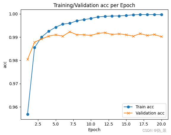
import matplotlib.pyplot as pltf, ax = plt.subplots()
ax.plot([None] + hist.history['accuracy'], 'o-')
ax.plot([None] + hist.history['val_accuracy'], 'x-')
# 绘制图例并自动使用最佳位置： loc = 0。
ax.legend(['Train acc', 'Validation acc'], loc = 0)
ax.set_title('Training/Validation acc per Epoch')
ax.set_xlabel('Epoch')
ax.set_ylabel('acc')
plt.show()

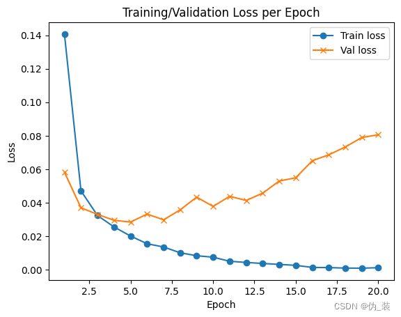
import matplotlib.pyplot as pltf, ax = plt.subplots()
ax.plot([None] + hist.history['loss'], 'o-')
ax.plot([None] + hist.history['val_loss'], 'x-')# Plot legend and use the best location automatically: loc = 0.
ax.legend(['Train loss', "Val loss"], loc = 0)
ax.set_title('Training/Validation Loss per Epoch')
ax.set_xlabel('Epoch')
ax.set_ylabel('Loss')
plt.show()