SQL

问题描述

SQL， 请根据前一周各产品的总GMV将其分成五类：GMV Top 20%、20%-40%，40%-60%，60%-80%以及Bottom 20%的产品组，请计算这五类产品组在后一周相较于前一周GMV的环比提升幅度

• 数据库中表名为 tmp_data
• 表字段：pID(产品名称), dID(销售日期，YYYY-MM-DD格式), gmv(金额)
• 假设数据连续且完整，即前后两周每日销售额没有为0的情况
  实现语言为SQL，最终请提交代码与计算结果

select min(dID), max(dID) from test_sql;#2022-10-29	2022-11-11select t1.lable, concat(round((t2.recent_week_gmv-t1.last_week_gmv)/t1.last_week_gmv,2),'%') as wow
from (select lable, sum(gmv_) as last_week_gmv
from (select pID, gmv_,
(case when rn<0.2 then 'Top 20%'
when rn<0.4 then '20%-40%'
when rn<0.6 then '40%-60%'
when rn<0.8 then '60%-80%'
else 'Bottom 20%' end) as lable
from 
(select pID, sum(gmv) as gmv_, cume_dist() over(order by sum(gmv) desc) as rn
from tmp_data
where dID>='2022-10-29' and dID<='2022-11-04'
group by pID
order by gmv_ desc) as a
) as b
group by lable
) as t1inner join (select lable, sum(gmv_) as recent_week_gmv
from (select pID, gmv_,
(case when rn<0.2 then 'Top 20%'
when rn<0.4 then '20%-40%'
when rn<0.6 then '40%-60%'
when rn<0.8 then '60%-80%'
else 'Bottom 20%' end) as lable
from 
(select pID, sum(gmv) as gmv_, cume_dist() over(order by sum(gmv) desc) as rn
from tmp_data
where dID>='2022-11-05' and dID<='2022-11-11'
group by pID
order by gmv_ desc) as a
) as b
group by lable
) as t2
on t2.lable = t1.lable;lable wow
Top 20%	-0.72%
20%-40%	-0.58%
40%-60%	-0.65%
60%-80%	-0.42%
Bottom 20%	-0.46%

python

问题描述

附件数据集(conversion_data.csv)为某平台用户转化信息。最终业务目标为提升转化率，希望分析团队通过数据分析、概率统计方法或机器学习方法给业务方相应的建议。

• 表中grpID为分组信息，base为该分组量级，cvr为该分组转化率（核心目标），feature1-feature28为统计到的28个影响特征

实现语言Python和R二选一，最终交付请包括注释、代码、输出、图表等可以展示分析思路与流程的内容，同时将Notebook转化成PDF格式再提交。

关于如何提升转化率，关键是找出哪些特征因子对cvr有正性影响，哪些对cvr有负性影响，其各自的影响程度分别是多少，通过扩大正性影响，降低负性影响从而达到提升转化率的效果，问题转化为去寻找特征因子对cvr的影响。具体可以先计算出各特征与cvr的pearson相关系数，再看看系数的热力图，再通过搭建模型查看各特征因子的在模型下对cvr的重要程度。

相关系数矩阵&热力图

Corr=df.corr() #相关系数矩阵
cor = Corr.sort_values(by = ['cvr'], axis=0, ascending = True) #按cvr排序横向排列
sns.heatmap(Corr, vmax=.8, square=True,) #热力图
plt.show()

               base       cvr  Feature1  Feature2  Feature3  ...  Feature24  Feature25  Feature26  Feature27  Feature28
Feature6   0.224114 -0.756728 -0.808393 -0.181685  0.288669  ...  -0.352540  -0.726383  -0.769274   0.566497   0.109772
Feature27  0.713999 -0.703784 -0.678812 -0.267156  0.332391  ...  -0.079622  -0.656632  -0.682684   1.000000  -0.010947
Feature3   0.478730 -0.534602 -0.517856 -0.988208  1.000000  ...   0.322946  -0.556814  -0.411315   0.332391   0.601913
Feature19  0.119104 -0.517936 -0.585010 -0.224186  0.281394  ...  -0.565172  -0.476672  -0.562676   0.343562  -0.180092
Feature7   0.370844 -0.474294 -0.196186  0.110337 -0.039697  ...  -0.158661  -0.108217  -0.143505   0.476188  -0.495868
Feature10  0.577230 -0.449998 -0.503034 -0.905145  0.891294  ...   0.310175  -0.551352  -0.474629   0.487161   0.658157
base       1.000000 -0.441421 -0.392978 -0.471431  0.478730  ...   0.068126  -0.376921  -0.375078   0.713999   0.178519
Feature18  0.077272 -0.203571 -0.236679  0.490290 -0.408194  ...  -0.220825  -0.208170  -0.276678   0.254997  -0.086524
Feature28  0.178519 -0.183497 -0.214614 -0.640599  0.601913  ...   0.655401  -0.336748  -0.198847  -0.010947   1.000000
Feature22  0.004151 -0.177423 -0.279160  0.354691 -0.290391  ...  -0.073605  -0.297561  -0.361559   0.181035   0.201477
Feature23 -0.160149 -0.108619 -0.093559  0.484322 -0.411309  ...   0.175318  -0.136582   0.068336   0.011303  -0.206764
Feature9   0.118227 -0.059924 -0.003391  0.244152 -0.222774  ...  -0.589892   0.108395  -0.172524   0.066214  -0.267187
Feature24  0.068126 -0.018481  0.118036 -0.373320  0.322946  ...   1.000000  -0.054716   0.229332  -0.079622   0.655401
Feature14 -0.081404  0.026290  0.010087 -0.241803  0.230874  ...   0.541626  -0.077957   0.182030  -0.021916   0.184277
Feature16  0.258838  0.070469  0.312441 -0.116694  0.075583  ...  -0.239778   0.400829   0.201863  -0.013232  -0.215665
Feature20 -0.196267  0.171468  0.081339  0.106536 -0.106389  ...  -0.170723   0.123204   0.053974   0.066488  -0.168935
Feature12 -0.268578  0.175629  0.158582  0.893915 -0.871301  ...  -0.477747   0.230034  -0.013711   0.031699  -0.575051
Feature5   0.342802  0.216372  0.380177 -0.070081  0.029075  ...   0.181418   0.354419   0.398978  -0.087208  -0.211474
Feature15  0.126423  0.227224  0.480034 -0.000748 -0.050945  ...  -0.206836   0.557642   0.376151  -0.176728  -0.283002
Feature21 -0.058053  0.309183  0.314857  0.097627 -0.118735  ...  -0.029046   0.338266   0.315115  -0.017281  -0.259533
Feature13 -0.580208  0.368426  0.340048  0.557234 -0.558035  ...   0.234146   0.247412   0.559932  -0.456297  -0.248982
Feature11 -0.553998  0.374911  0.410215  0.928251 -0.897625  ...  -0.375576   0.470418   0.379569  -0.406848  -0.677061
Feature2  -0.471431  0.437308  0.420028  1.000000 -0.988208  ...  -0.373320   0.469587   0.332699  -0.267156  -0.640599
Feature4  -0.408524  0.512194  0.762520  0.651733 -0.701479  ...  -0.180543   0.750906   0.481900  -0.507596  -0.452813
Feature17 -0.406211  0.790212  0.959055  0.460516 -0.540032  ...  -0.030287   0.986516   0.787931  -0.687834  -0.347838
Feature8  -0.408669  0.803202  0.961982  0.463937 -0.545872  ...  -0.037030   0.986828   0.785132  -0.691376  -0.341361
Feature26 -0.375078  0.816414  0.830065  0.332699 -0.411315  ...   0.229332   0.793896   1.000000  -0.682684  -0.198847
Feature25 -0.376921  0.840333  0.963762  0.469587 -0.556814  ...  -0.054716   1.000000   0.793896  -0.656632  -0.336748
Feature1  -0.392978  0.852769  1.000000  0.420028 -0.517856  ...   0.118036   0.963762   0.830065  -0.678812  -0.214614
cvr       -0.441421  1.000000  0.852769  0.437308 -0.534602  ...  -0.018481   0.840333   0.816414  -0.703784  -0.183497

从相关系数矩阵可以看到从小到大的排列和取值如下表所示

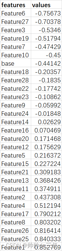
从Pearson相关系数来看，values值大于0.7的有Feature1,Feature25,Feature26,Feature8,Feature17,Feature6,Feature27一共7个，我们可以利用feature_selection来进一步验证。

feature_selection

直接调用sklearn的feature_selection类也是可以找出这7个最为重要的特征变量的，然而在现实生活中我们选择特征个数不能单单只要这7个就够了，我们可以适当的放缩一些，比如9个，10个，11个等，然后再把这些特征摘出来做建模准备。

selector = SelectKBest(f_regression, k=9)
z = selector.fit_transform(X, y)
filter = selector.get_support()
features = np.array(X.columns) #所有特征变量名
print("筛选出来的9个特征变量名:{}".format(features[filter])) #筛选出的特征变量

输出

选出来的9个特征变量名:['Feature1' 'Feature3' 'Feature6' 'Feature8' 'Feature17' 'Feature19''Feature25' 'Feature26' 'Feature27']

其实，这个时候从结果来看已经能够看出一二了，可以结合具体业务给出哪些指标应该的加强的，哪些指标应该抑制的。

预测模型

作为数据科学家应该利用已有的历史数据为未来的变动给出具有指导性预测，这种场景往往发生在某些变量明确会在未来一段时间内发生明显变化，如计划在未来2周内加大线上广告投入资金，所以我们需要根据某些变量的变化来预测未来转化率的变化情况，需要进行预测模型搭建，针对这些量化很好的结构型数据，现在比较流行的做法是先做一个简单的模型，观看其效果，然后再用一些魔改的集成学习算法，下面以GBDT算法为例来进行预测模型搭建。

X, y =  df[['Feature1', 'Feature3', 'Feature6', 'Feature8', 'Feature17', 'Feature19','Feature25', 'Feature26', 'Feature27']], df.cvr #特征和目标
X_train, X_test, y_train, y_test = train_test_split(X, y, test_size = 0.3, shuffle=True, random_state=0) #划分训练测试集
less_cat_col = [col_name for col_name in X_train.columns if X_train[col_name].dtype=='object' and X_train[col_name].nunique()<10] #少类别型变量
more_cat_col = [col_name for col_name in X_train.columns if X_train[col_name].dtype=='object' and X_train[col_name].nunique()>=10] #多类别型变量
num_col = [col_name for col_name in X_train.columns if X_train[col_name].dtype in ['int64', 'float64']] #数值型特征
# print(less_cat_col, more_cat_col, num_col)less_cat_transform = Pipeline(steps = [('imputer', SimpleImputer(strategy='most_frequent')),('encoder', OneHotEncoder(handle_unknown='ignore'))]) #类别型变量先用众数填充再独热编码
more_cat_transform = Pipeline(steps = [('imputer', SimpleImputer(strategy='most_frequent')),('encoder', OrdinalEncoder(handle_unknown='use_encoded_value', unknown_value=-1))]) #类别型变量先用众数填充再普通编码num_transform = Pipeline(steps = [('imputer', SimpleImputer(strategy='mean')),('scaler', StandardScaler())]) #数值型变量采用均值填充和标准化
preprocessor = ColumnTransformer(transformers = [('less_cat', less_cat_transform, less_cat_col),('more_cat', more_cat_transform, more_cat_col),('num', num_transform, num_col)]) #不同的预处理步骤打包到一起
model = GradientBoostingRegressor(n_estimators = 300, learning_rate = 0.05, max_depth = 7,  min_samples_leaf= 3, random_state=0) # 模型初始化
pipe = Pipeline(steps=[('preprocessing', preprocessor),('model', model)])
pipe.fit(X_train, y_train)
y_pred = pipe.predict(X_test)
MAE = mean_absolute_error(y_test, y_pred) #平均绝对误差
score = pipe.score(X_test, y_test)
# print(pipe.named_steps['preprocessing']._feature_names_in)
# print(pipe.named_steps['preprocessing'].get_feature_names)
# print(pipe.named_steps['model'].feature_importances_)
print("mean_absolute_error: {}, and model score: {}".format(MAE, score))
with open(r"D:\项目\acxiom的面试\模型测试 A\有工作经验\conversation.pickle", "wb") as model_file: #保存/data/model/pickle.dump(pipe, model_file)

最后模型2个重要的评估指标是

mean_absolute_error: 0.4527472563951145, and model score: 0.6817745289721121

其实，针对这种样本量偏小的模型得分接近0.7已经不错了，后续更应该注重数据积累和特征量化工作的pipeline。

开放性业务题（二选一）

问题描述

注：题目为开放性，可自由提出各种假设前提、设定问题边界等

1. 如何给某品牌所有消费者做价值分层？如何找到核心高价值消费者？如何发掘有潜力的消费者？
2. 电商大促活动如何有针对性的给不同用户发券？如何测试该策略是否对业务有提升？

这里简单回答一下第一个问题，首先，要界定客户价值，客户价值评估的维度，如果没有这方面的知识积累的话，可以参考经典RFM模型，从客户价值的最常用的三个维度来进行评估，有R（Recency）交易间隔、F（Frequency）交易频度、M（Monetary）交易金额，这三个维度是跨时间，可以提前约定时间跨度，比如1个月，3个月，半年，一年，3年等，这样做有其好处，然后将问题转化为聚类问题，可以将客户分成高价值，中价值，低价值三类客户，然后聚焦每一类客户主题的共性和差异性，哪些弱，哪些强，补弱扶强策略进行精准营销。

完整代码

# -*- encoding: utf-8 -*-
'''
@Project :   conversation
@Desc    :   提升转化率
@Time    :   2023/02/24 19:53:24
@Author  :   帅帅de三叔,zengbowengood@163.com
'''
import pickle
import numpy as np
import pandas as pd
import matplotlib.pyplot as plt
import seaborn as sns
from sklearn.preprocessing import MinMaxScaler
from sklearn.feature_selection import SelectKBest,f_regression
from sklearn.decomposition import PCA
from sklearn.model_selection import train_test_split, GridSearchCV
from sklearn.compose import ColumnTransformer
from sklearn.pipeline import Pipeline
from sklearn.preprocessing import  OneHotEncoder, OrdinalEncoder, StandardScaler
from sklearn.impute import SimpleImputer
from sklearn.ensemble import GradientBoostingRegressor
from sklearn.metrics import mean_absolute_error
conversation_data = pd.read_csv(r"D:\项目\acxiom的面试\模型测试 A\有工作经验\conversation_data.csv", delimiter = ',', index_col='grp_ID')
df=(conversation_data-conversation_data.mean())/conversation_data.std() #标准化
X,y = df.drop(labels=['cvr'], axis=1), df.cvr #特征变量，目标变量Corr=df.corr() #相关系数矩阵
cor = Corr.sort_values(by = ['cvr'], axis=0, ascending = True) #按cvr排序横向排列
sns.heatmap(Corr, vmax=.8, square=True,) #热力图
plt.show()selector = SelectKBest(f_regression, k=9) #准备筛选9个特征变量进行建模
z = selector.fit_transform(X, y)
filter = selector.get_support()
features = np.array(X.columns) #所有特征变量名
print("筛选出来的9个特征变量名:{}".format(features[filter])) #筛选出的特征变量X, y =  df[['Feature1', 'Feature3', 'Feature6', 'Feature8', 'Feature17', 'Feature19','Feature25', 'Feature26', 'Feature27']], df.cvr #特征和目标
X_train, X_test, y_train, y_test = train_test_split(X, y, test_size = 0.3, shuffle=True, random_state=0) #划分训练测试集
less_cat_col = [col_name for col_name in X_train.columns if X_train[col_name].dtype=='object' and X_train[col_name].nunique()<10] #少类别型变量
more_cat_col = [col_name for col_name in X_train.columns if X_train[col_name].dtype=='object' and X_train[col_name].nunique()>=10] #多类别型变量
num_col = [col_name for col_name in X_train.columns if X_train[col_name].dtype in ['int64', 'float64']] #数值型特征
# print(less_cat_col, more_cat_col, num_col)less_cat_transform = Pipeline(steps = [('imputer', SimpleImputer(strategy='most_frequent')),('encoder', OneHotEncoder(handle_unknown='ignore'))]) #类别型变量先用众数填充再独热编码
more_cat_transform = Pipeline(steps = [('imputer', SimpleImputer(strategy='most_frequent')),('encoder', OrdinalEncoder(handle_unknown='use_encoded_value', unknown_value=-1))]) #类别型变量先用众数填充再普通编码num_transform = Pipeline(steps = [('imputer', SimpleImputer(strategy='mean')),('scaler', StandardScaler())]) #数值型变量采用均值填充和标准化
preprocessor = ColumnTransformer(transformers = [('less_cat', less_cat_transform, less_cat_col),('more_cat', more_cat_transform, more_cat_col),('num', num_transform, num_col)]) #不同的预处理步骤打包到一起
model = GradientBoostingRegressor(n_estimators = 300, learning_rate = 0.05, max_depth = 7,  min_samples_leaf= 3, random_state=0) # 模型初始化
pipe = Pipeline(steps=[('preprocessing', preprocessor),('model', model)])
pipe.fit(X_train, y_train)
y_pred = pipe.predict(X_test)
MAE = mean_absolute_error(y_test, y_pred) #平均绝对误差
score = pipe.score(X_test, y_test)
# print(pipe.named_steps['preprocessing']._feature_names_in)
# print(pipe.named_steps['preprocessing'].get_feature_names)
# print(pipe.named_steps['model'].feature_importances_)
print("mean_absolute_error: {}, and model score: {}".format(MAE, score))
with open(r"D:\项目\acxiom的面试\模型测试 A\有工作经验\conversation.pickle", "wb") as model_file: #保存/data/model/pickle.dump(pipe, model_file)