[动手学深度学习]生成对抗网络GAN学习笔记
论文原文:Generative Adversarial Nets (neurips.cc)
李沐GAN论文逐段精读:GAN论文逐段精读【论文精读】_哔哩哔哩_bilibili
论文代码:http://www.github.com/goodfeli/adversarial
Ian, J. et al. (2014) 'Generative adversarial network', NIPS'14: Proceedings of the 27th International Conference on Neural Information Processing Systems, Vol. 2, pp 2672–2680. doi: https://doi.org/10.48550/arXiv.1406.2661
目录
1. GAN论文原文学习
1.1. Abstract
1.2. Introduction
1.3. Related work
1.4. Adversarial nets
1.5. Theoretical Results
1.5.1. Global Optimality of p_g = p_data
1.5.2. Convergence of Algorithm 1
1.6. Experiments
1.7. Advantages and disadvantages
1.8. Conclusions and future work
2. 知识补充
2.1. Divergence
2.2. 唠嗑一下
1. GAN论文原文学习
1.1. Abstract
①They combined generative model and discriminative model
together, which forms a new model.
is the "cheating" part which focus on imitating and
is the "distinguishing" part which focus on distinguishing where the data comes from.
②This model is rely on a "minmax" function
③GAN does not need Markov chains or unrolled approximate inference nets
④They designed qualitative and quantitative evaluation to analyse the feasibility of GAN
1.2. Introduction
①The authors praised deep learning and briefly mentioned its prospects
②Due to the difficulty of fitting or approximating the distribution of the ground truth, the designed a new generative model
③They compare the generated model to the person who makes counterfeit money, and the discriminative model to the police. Both parties will mutually promote and grow. The authors ultimately hope that the ability of the counterfeiter can be indistinguishable from the genuine product
④Both and
are MLP, and
passes random noise
⑤They just adopt backpropagation and dropout in training
corpora 全集;corpus 的复数
counterfeiter n.伪造者;制假者;仿造者
1.3. Related work
①Recent works are concentrated on approximating function, such as succesful deep Boltzmann machine. However, their likelihood functions are too complex to process.
②Therefore, here comes generative model, which only generates samples but does not approximates function. Generative stochastic networks are an classic generative model.
③Their backpropagation:
④Variational autoencoders (VAEs) in Kingma and Welling and Rezende et al. do the similar work. However, VAEs are modeled by differentiate hidden units, which is contrary to GANs.
⑤And some others aims to approximate but are hard to. Such as Noise-contrastive estimation (NCE), discriminating data under noise, but limited in its discriminator.
⑥The most relevant work is predictability minimization, it utilize other hiden units to predict given unit. However, PM is different from GAN in that (a) PM focus on objective function minimizing, (b) PM is just a regularizer, (c) the two networks in PM respectively make output similar or different
⑦Adversarial examples distinguish which data is misclassified with no generative function
1.4. Adversarial nets
①They designed a minimax function:
where denotes generator's distribution,
represents data,
denotes prior probability with noise,
denotes a differentiable function, namely a MLP layer, with parameters
,
also denotes a MLP layer with its output is a scalar, where the scalar is the probability that
is real data exceeds the probability that it is generated data
②They train and
together with maximizing
and minimizing
③They reckon is more likely to be overfitting. Hence, k-steps of optimizing
and 1-step optimizing of
is more suitable
④ is relatively weak in early stages, thus train
first might achieve better results
pedagogical adj.教育学的;教学论的
1.5. Theoretical Results
①Their fitting diagram:
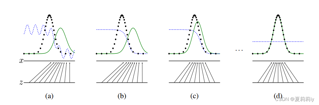
where is blue and dashed line,
is green and solid line, the real data distribution is black and dashed line,
converges to
. And when it equals to
with
that means
can not discriminate any data
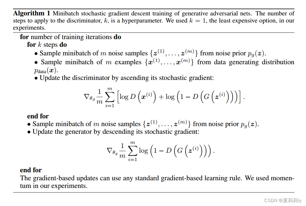
②Pseudocode of GAN:
1.5.1. Global Optimality of p_g = p_data
①They need to maximize for
:
for any coefficient , the value of expression
achieves its maximum when
. Thus
②Then change the original function to:
③ is the minimum of
when
④KL divergence used for it:
⑤JS divergence used for it:
and the authors recognized the non negative nature of JS divergence more, therefore adopting JS divergence
1.5.2. Convergence of Algorithm 1
①The function is convex so that when gradient updating tends to stabilize, it may achieve the global optima
②Parzen window-based log-likelihood estimates:
where they adopt mean loglikelihood of samples on MNIST, standard error across folds of TFD
supremum n.上确界;最小上界;上限
1.6. Experiments
①Datasets: MNIST, Toronto Face Database (TFD), CIFAR-10
②Activation: combination of ReLU and Sigmoid for generator, Maxout for discriminator
③Adopting dropout in discriminator
④Noise is only allowed as the bottommost input
⑤Their Gaussian Parzen window method brings high variance and performs somewhat poor in high dimensional spaces
1.7. Advantages and disadvantages
(1)Disadvantages
①There is no clear representation of
②It is difficult to achieve synchronous updates between and
(2)Advantages
①No need for Markov chain
②Updating by gradients instead of data
③They can express any distribution
1.8. Conclusions and future work
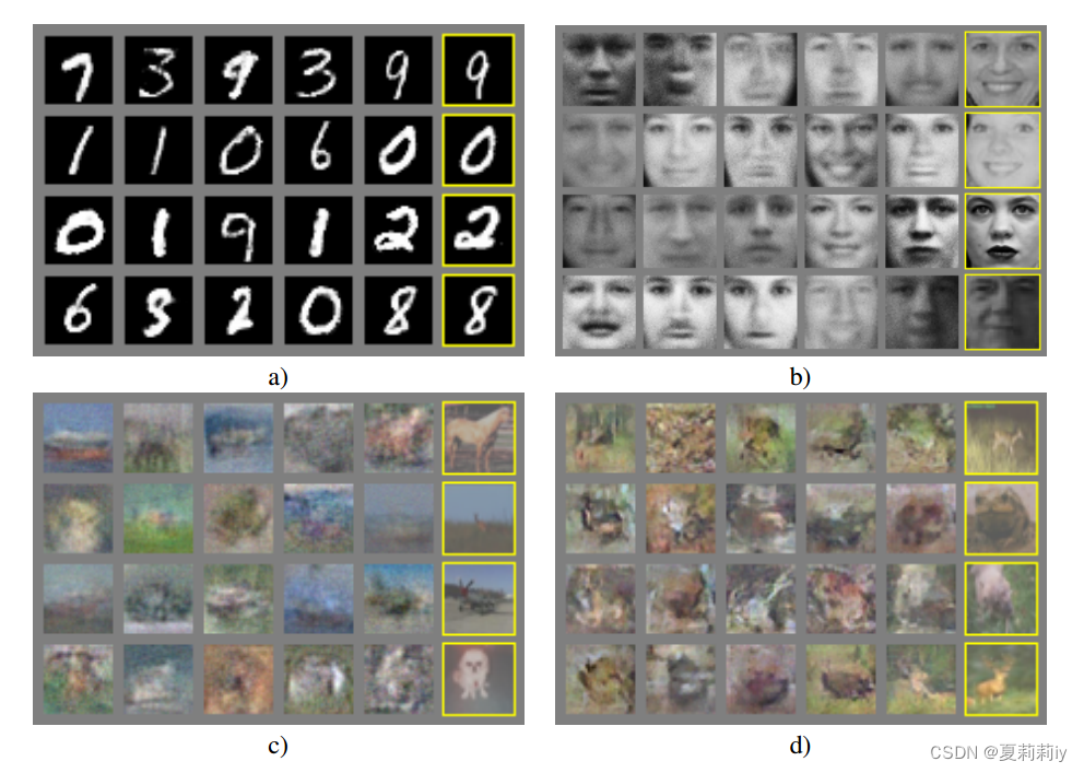
①Samples (left) and generative data (right with yellow outlines) in (a) MNIST, (b) TFD, (c) CIFAR-10 (fully connected model), (d) CIFAR-10 (convolutional discriminator and “deconvolutional” generator):
②"Digits obtained by linearly interpolating between coordinates in space of the full model":

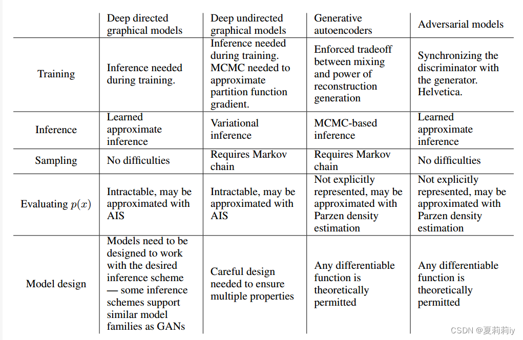
③Their summary of challenges in different parts:
interpolate v.〈数〉插(值),内插,内推;计算(中间值);插入(字句等);添加(评论或字句);篡改;插话,插嘴
2. 知识补充
2.1. Divergence
(1)Kullback–Leibler divergence (KL divergence)
①相关链接:机器学习:Kullback-Leibler Divergence (KL 散度)_kullback-leibler散度-CSDN博客
②关于KL散度(Kullback-Leibler Divergence)的笔记 - 知乎 (zhihu.com)
(2)Jensen–Shannon divergence (JS divergence)
①理解JS散度(Jensen–Shannon divergence)-CSDN博客
2.2. 唠嗑一下
(1)论文倒是精简易懂,特别是配上李沐的讲解之后更没啥大问题了。但是作者提供的源码还是有点过于爆炸,且README没有多说。很难上手啊,新人完全不推荐