【深度学习实验】数据可视化
目录
一、实验介绍
二、实验环境
三、实验内容
0. 导入库
1. 归一化处理
归一化
实验内容
2. 绘制归一化数据折线图
报错
解决
3. 计算移动平均值SMA
移动平均值
实验内容
4. 绘制移动平均值折线图
5 .同时绘制两图
6. array转换为tensor张量
7. 打印张量
一、实验介绍
Visualizing the Trend of Random Data Changes可视化随机数据变化的趋势
二、实验环境
conda create -n DL python=3.7 conda activate DLpip install torch==1.8.1+cu102 torchvision==0.9.1+cu102 torchaudio==0.8.1 -f https://download.pytorch.org/whl/torch_stable.html
conda install matplotlib
三、实验内容
0. 导入库
According to the usual convention, import numpy, matplotlib.pyplot, and torch.按照通常的惯例,导入 numpy、matplotlib.pyplot 和 torch。
import numpy as np
import matplotlib.pyplot as plt
import torch
1. 归一化处理
归一化
归一化处理是一种常用的数据预处理技术,用于将数据缩放到特定的范围内,通常是[0,1]或[-1,1]。这个过程可以确保不同特征或指标具有相似的数值范围,避免某些特征对模型训练的影响过大。
在机器学习和数据分析中,归一化可以帮助改善模型的收敛速度和性能,减少由于特征尺度差异导致的问题。例如,某些机器学习算法(如梯度下降)对特征的尺度敏感,如果不进行归一化处理,可能会导致模型难以收敛或产生不准确的结果。
常用的归一化方法包括最小-最大归一化(Min-Max normalization)和Z-score归一化(标准化)。
- 最小-最大归一化将数据线性地缩放到指定的范围内。
- Z-score归一化通过计算数据的均值和标准差,将数据转换为均值为0,标准差为1的分布。
实验内容
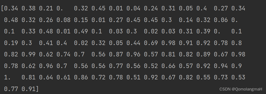
Read the file named `data.txt` containing 100 integers using NumPy, normalize all values to the range [0, 1], and store the normalized array with two decimal places.
使用 NumPy 读取包含 100 个整数的名为“data.txt”的文件,将所有值规范化为范围 [0, 1],并存储具有两个小数位的规范化数组。
data = np.loadtxt('data.txt')
# 归一化处理
normalized_array = (data - np.min(data)) / (np.max(data) - np.min(data))
# 保留两位小数
normalized_data = np.round(normalized_array, 2)
# 打印归一化后的数组
print(normalized_array)
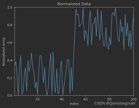
2. 绘制归一化数据折线图
Create a line plot using Matplotlib where the x-axis represents the indices of the normalized array ranging from 1 to 100, and the y-axis represents the values of the normalized array ranging from 0 to 1.
使用 Matplotlib 创建一个折线图,其中 x 轴表示规范化数组的索引,范围从1到100,y 轴表示规范化数组的值,范围从0到1。
# 创建x轴数据
x = np.arange(1, 101)
# 绘制折线图
plt.plot(x, normalized_array)# 设置x轴和y轴的范围
plt.xlim(1, 100)
plt.ylim(0, 1)
plt.title("Normalized Data")
plt.xlabel("Index")
plt.ylabel("Normalized Array")
plt.show()
报错
OMP: Error #15: Initializing libiomp5md.dll, but found libiomp5md.dll already initialized.
OMP: Hint This means that multiple copies of the OpenMP runtime have been linked into the program. That is dangerous, since it can degrade performance or cause incorrect results. The best thing to do is to ensure that only a single OpenMP runtime is linked into the process, e.g. by avoiding static linking of the OpenMP runtime in any library. As an unsafe, unsupported, undocumented workaround you can set the environment variable KMP_DUPLICATE_LIB_OK=TRUE to allow the program to continue to execute, but that may cause crashes or silently produce incorrect results. For more information, please see http://www.intel.com/software/products/support/.
解决
conda install nomkl
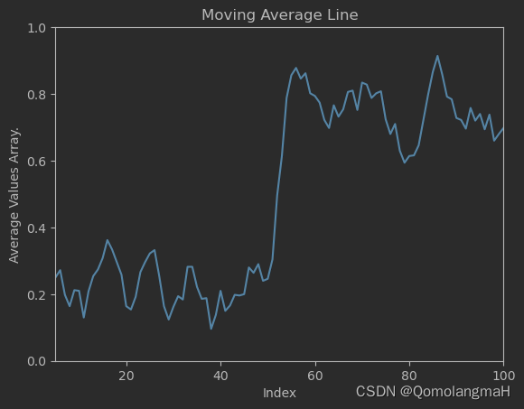
3. 计算移动平均值SMA
移动平均值
移动平均值(Moving Average)是一种数据平滑处理的方法,可以在一段时间内计算数据序列的平均值。这种方法通过不断更新计算的平均值,使得输出的数据更加平滑,减少噪声和突变的影响。
移动平均值有多种类型,其中最常见的是简单移动平均值(Simple Moving Average,SMA)和指数移动平均值(Exponential Moving Average,EMA)。这两种方法的计算方式略有不同。
-
简单移动平均值(SMA):
简单移动平均值是对指定时间段内的数据进行平均处理的方法,计算公式如下:SMA = (X1 + X2 + X3 + ... + Xn) / n其中,X1, X2, ..., Xn 是指定时间段内的数据,n 是时间段的长度。
例如,要计算最近5天的简单移动平均值,可以将这5天的数据相加,再除以5。
-
指数移动平均值(EMA):
指数移动平均值是对数据进行加权平均处理的方法,计算公式如下:EMA = (X * (2/(n+1))) + (EMA_previous * (1 - (2/(n+1))))其中,X 是当前数据点的值,n 是时间段的长度,EMA_previous 是上一个时间段的指数移动平均值。
指数移动平均值使用了指数衰减的加权系数,更加重视最近的数据点。
使用移动平均值可以平滑数据序列,使得数据更具可读性,减少随机波动的影响。这在时间序列分析、技术分析和数据预测等领域经常被使用。
实验内容
Calculate the moving average of the normalized results using NumPy with a window size of 5. Store the calculated moving average values in a new one-dimensional NumPy array, referred to as the "average values array."
使用窗口大小为 5 的 NumPy 计算归一化结果的移动平均值。将计算出的移动平均值存储在新的一维 NumPy 数组(称为“平均值数组”)中。
# 计算移动平均值
average_values_array = np.convolve(normalized_array, np.ones(5)/5, mode='valid')
print(average_values_array)
4. 绘制移动平均值折线图
Create another line plot using Matplotlib where the x-axis represents the indices of the average values array ranging from 5 to 100, and the y-axis represents the values of the average values array ranging from 0 to 1.
使用 Matplotlib 创建另一个线图,其中 x 轴表示平均值数组的索引,范围从 5 到 100,y 轴表示从 0 到 1 的平均值数组的值。
x_axis = range(5, 101)# 绘制折线图
plt.plot(x_axis, average_values_array)plt.xlim(5, 100)
plt.ylim(0, 1)
plt.title('Moving Average Line')
plt.xlabel('Index')
plt.ylabel('Average Values Array.')
plt.show()
5 .同时绘制两图
Combine the line plots of the normalized array and the average values array in the same figure using different colors for each line.
将归一化数组的线图和平均值数组组合在同一图中,每条线使用不同的颜色。
plt.plot(x, normalized_array, color='r', label='Normalized Array Line')
plt.plot(x_axis, average_values_array, color='b', label='Moving Average Line')
plt.legend()
plt.xlim(1, 100)
plt.ylim(0, 1)
plt.xlabel('Index')
plt.ylabel('Value')
plt.show()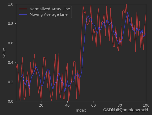
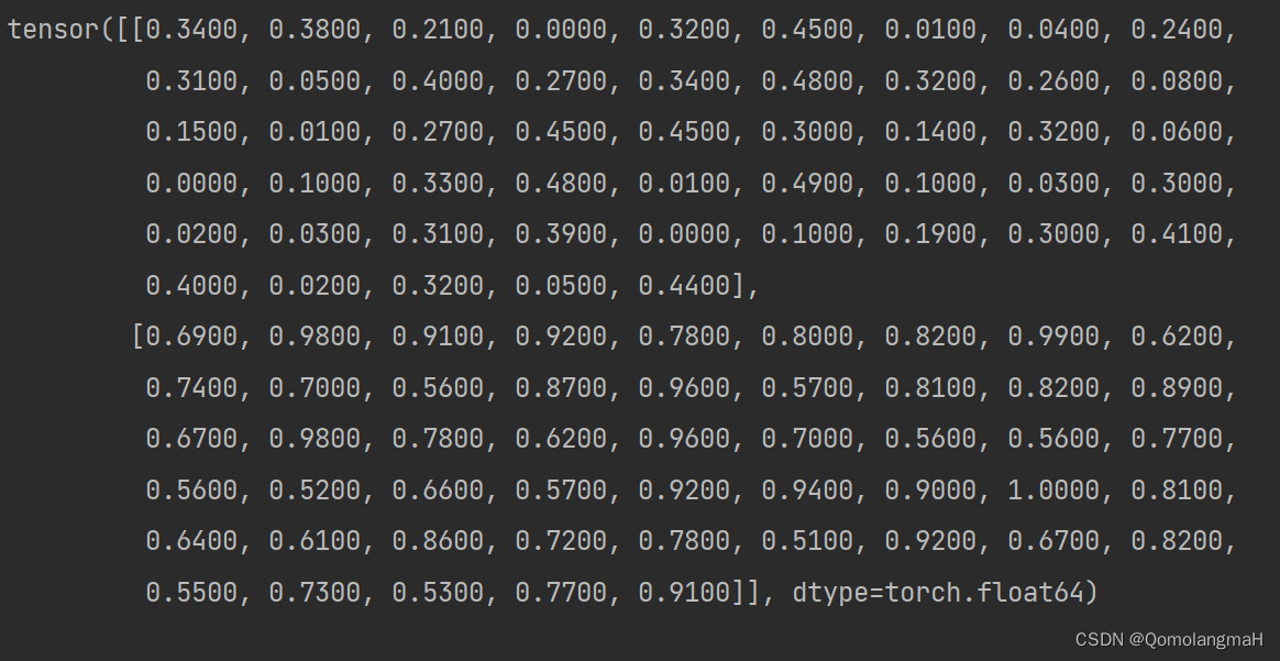
6. array转换为tensor张量
Transform the normalized array into a 2x50 Tensor by reshaping the data.
通过重塑数据将归一化数组转换为 2x50 张量。
normalized_tensor = torch.tensor(normalized_array).reshape(2, 50)
7. 打印张量
Print the resulting Tensor.
print(normalized_tensor)