• 🍨 本文为🔗365天深度学习训练营 中的学习记录博客
• 🍦 参考文章：Pytorch实战 | 第P5周：运动鞋识别
• 🍖 原作者：K同学啊 | 接辅导、项目定制
• 🚀 文章来源：K同学的学习圈子

---

---

环境

• 系统: Linux
• 语言: Python3.8.10
• 深度学习框架: Pytorch2.0.0+cu118

---

步骤

环境设置

包引用

import torch
import torch.nn as nn 
import torch.optim as optim # 优化器
import torch.nn.functional as F # 可以静态调用的方法from torchvision import datasets, transforms # 数据集创建、数据预处理方法
from torch.utils.data import DataLoader # DataLoader可以将数据集封装成批次数据import matplotlib.pyplot as plt
import numpy as np
from PIL import Image # 加载图片预览使用的库
from torchinfo import summary # 可以打印模型实际运行时的图
import copy # 深拷贝使用的库
import pathlib, random # 文件夹遍历和随机数

训练设备

# 声明一个全局设备对象，方便后面将数据和模型拷贝到设备中
device = torch.device('cuda' if torch.cuda.is_available() else 'cpu')

数据准备

图像解压后的路径

train_path = 'train'
test_path = 'test'

打印图像的参数

train_pathlib = pathlib.Path(train_path)
train_image_list = list(train_pathlib.glob('*/*'))
for _ in range(5):print(np.array(Image.open(str(random.choice(train_image_list)))).shape)

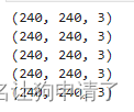
重复执行了多次，返回结果都是(240, 240, 3)，可以确定图像的大小统一为240,240，在数据加载的过程中可以不对图像做缩放处理。

展示图像

plt.figure(figsize=(20, 4))
for i in range(20):image = random.choice(train_image_list)plt.subplot(2, 10, i+1)plt.axis('off')plt.imshow(Image.open(str(image)))plt.title(image.parts[-2])

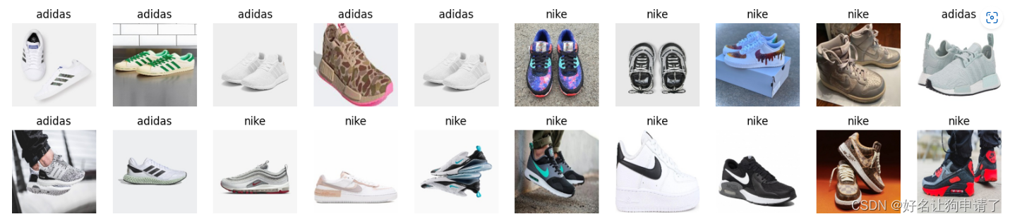
至此我们对数据集中的图像有了一个初步的了解。接下来就是准备训练数据。

图像的预处理

定义一些图像的预处理方法，例如将图像读取并转为pytorch的tensor对象，然后对图像的数值做归一化处理

transform = transforms.Compose([transforms.ToTensor(),transforms.Normalize(mean=[0.485, 0.456, 0.406], std=[0.229, 0.224, 0.225])
])

创建数据集

train_dataset = datasets.ImageFolder(train_path, transform=transform)
test_dataset = datasets.ImageFolder(test_path, transform=transform)

获取数据集的分类

class_names = [key for key in train_dataset.class_to_idx]
print(class_names)

打乱数据的顺序，生成批次

batch_size = 32
train_loader = DataLoader(train_dataset, shuffle=True, batch_size=batch_size)
test_loader = DataLoader(test_dataset, batch_size=batch_size)

模型设计

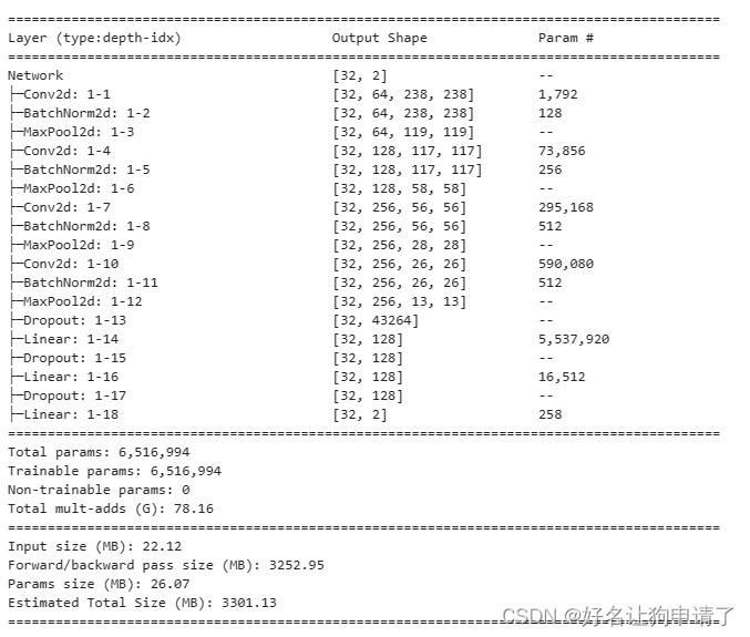
使用3x3的卷积核，最大的通道数到256，每次卷积操作后，就紧跟一个池化层，一共使用了4个卷积层和4个池化层。最后使用了三层全连接网络来做分类器。

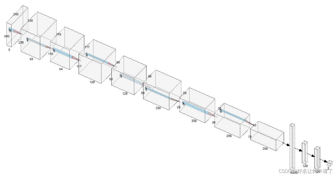
class Network(nn.Module):def __init__(self, num_classes):super().__init__()self.conv1 = nn.Conv2d(3, 64, 3)self.bn1  = nn.BatchNorm2d(64)self.conv2 = nn.Conv2d(64, 128, 3)self.bn2 = nn.BatchNorm2d(128)self.conv3 = nn.Conv2d(128, 256, 3)self.bn3 = nn.BatchNorm2d(256)self.conv4 = nn.Conv2d(256, 256, 3)self.bn4 = nn.BatchNorm2d(256)self.maxpool = nn.MaxPool2d(2)self.fc1 = nn.Linear(13*13*256, 128)self.fc2 = nn.Linear(128, 128)self.fc3 = nn.Linear(128, num_classes)self.dropout = nn.Dropout(0.5)def forward(self, x):# 240 -> 238x = F.relu(self.bn1(self.conv1(x)))# 238 -> 119x = self.maxpool(x)# 119 -> 117x = F.relu(self.bn2(self.conv2(x)))# 117 -> 58x = self.maxpool(x)# 58 -> 56x = F.relu(self.bn3(self.conv3(x)))# 56 -> 28x = self.maxpool(x)# 28 -> 26x = F.relu(self.bn4(self.conv4(x)))# 26 -> 13x = self.maxpool(x)x = x.view(x.size(0), -1)x = self.dropout(x)x = F.relu(self.dropout(self.fc1(x)))x = F.relu(self.dropout(self.fc2(x)))x = self.fc3(x)return x
model = Network(len(class_names)).to(device)summary(model, input_size=(32, 3, 240, 240))

模型训练

模型训练过程中，每个epoch都会对全部的训练集进行一次完整的遍历，所以可以封装一些训练和评估方法，将业务逻辑和循环分开

训练函数

def train(train_loader, model, loss_fn, optimizer):size = len(train_loader.dataset)num_batches = len(train_loader)train_loss, train_acc = 0, 0for x, y in train_loader:x, y = x.to(device), y.to(device)pred = model(x)loss = loss_fn(pred, y)optimizer.zero_grad()loss.backward()optimizer.step()train_loss += loss.item()train_acc += (pred.argmax(1) == y).type(torch.float).sum().item()train_loss /= num_batchestrain_acc /= sizereturn train_loss, train_acc

评估函数

def test(test_loader, model, loss_fn):size = len(test_loader.dataset)num_batches = len(test_loader)test_loss, test_acc = 0, 0for x, y in test_loader:x, y = x.to(device), y.to(device)pred = model(x)loss = loss_fn(pred, y)test_loss += loss.item()test_acc += (pred.argmax(1) == y).type(torch.float).sum().item()test_loss /= num_batchestest_acc /= sizereturn test_loss, test_acc

循环迭代部分

loss_fn = nn.CrossEntropyLoss()
optimizer = optim.Adam(model.parameters(), lr=1e-4)
scheduler = optim.lr_scheduler.LambdaLR(optimizer=optimizer, lr_lambda=lambda epoch:0.92**(epoch //2)) 
# 创建学习率的衰减
epochs = 50train_loss, train_acc = [], []
test_loss, test_acc = [], []
best_acc = 0
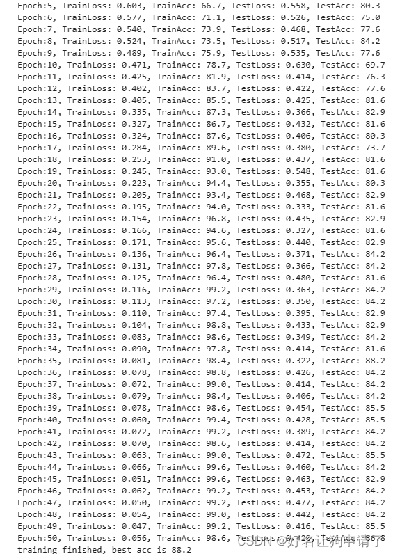
for epoch in range(epochs):model.train()epoch_train_loss, epoch_train_acc = train(train_loader, model, loss_fn, optimizer)model.eval()with torch.no_grad():epoch_test_loss, epoch_test_acc = test(test_loader, model, loss_fn)scheduler.step() # 每次迭代调用一次，自动做学习率衰减# 如果当前评估的学习率更好，就保存当前模型if best_acc < epoch_test_acc:best_acc = epoch_test_accbest_model = copy.deepcopy(model)# 记录历史记录train_loss.append(epoch_train_loss)train_acc.append(epoch_train_acc)test_loss.append(epoch_test_loss)test_acc.append(epoch_test_acc)# 打印每个迭代的数据print(f"Epoch:{epoch+1}, TrainLoss: {epoch_train_loss:.3f}, TrainAcc: {epoch_train_acc*100:.1f}, TestLoss: {epoch_test_loss:.3f}, TestAcc: {epoch_test_acc*100:.1f}")# 打印本次训练的最佳正确率
print(f'training finished, best_acc is {best_acc*100:.1f}')# 将最佳模型保存到文件中
torch.save(model.state_dict(), 'best_model.pth')

模型效果展示

训练过程图表展示

画一个拆线图，观察训练过程中损失函数和正确率的变化趋势

plt.figure(figsize=(20,5))epoch_range = range(epochs)plt.subplot(1,2, 1)
plt.plot(epoch_range, train_loss, label='train loss')
plt.plot(epoch_range, test_loss, label='validation loss')
plt.legend(loc='upper right')
plt.title('Loss')plt.subplot(1,2,2)
plt.plot(epoch_range, train_acc, label='train accuracy')
plt.plot(epoch_range, test_acc, label='validation accuracy')
plt.legend(loc='lower right')
plt.title('Accuracy')

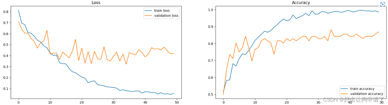
可以看出模型在最后基本已经收敛，最佳准确率是88.2%，满足了挑战任务。

载入最佳模式，随机选择图像进行预测

model.load_state_dict(torch.load('best_model.pth'))
model = model.to(device)test_pathlib = pathlib.Path(test_path)image_list = list(test_pathlib.glob('*/*'))image_path = random.choice(image_list)
image = transform(Image.open(str(image_path)))
image = image.unsqueeze(0)
image = image.to(device)pred = model(image)plt.figure(figsize=(5,5))
plt.axis('off')
plt.imshow(Image.open(str(image_path)))
plt.title(f'real: {image_path.parts[-2]}, predict: {class_names[pred.argmax(1).item()]}')

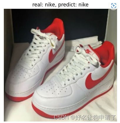
上次运行上面的预测任务，发现正确率还不错。

总结与心得体会

1. 整个模型设计的思路其实是模仿了vgg16模型，在卷积层的数量和通道上做了简化。轻量级的任务可以首先试着减少池化层间的卷积次数，减少模型中最大的特征图的通道数
2. 对图像的归一化操作很重要。在没有归一化前，模型的最佳正确率只能达到80%，推测可能是因为未做归一化的图像值域范围太大，不方便收敛，归一化后，原始图像中的输入特征值范围变成0~1,模型的权重变化更易作用到特征上。