数学建模及数据分析 || 4. 深度学习应用案例分享
PyTorch 深度学习全连接网络分类
文章目录
- PyTorch 深度学习全连接网络分类
- 1. 非线性二分类
- 2. 泰坦尼克号数据分类
- 2.1 数据的准备工作
- 2.2 全连接网络的搭建
- 2.3 结果的可视化
1. 非线性二分类
import sklearn.datasets #数据集
import numpy as np
import matplotlib.pyplot as plt
from sklearn.metrics import accuracy_scoreimport torch
import numpy as np
import matplotlib.pyplot as plt
import torch.nn as nnnp.random.seed(0) #设置随机数种子
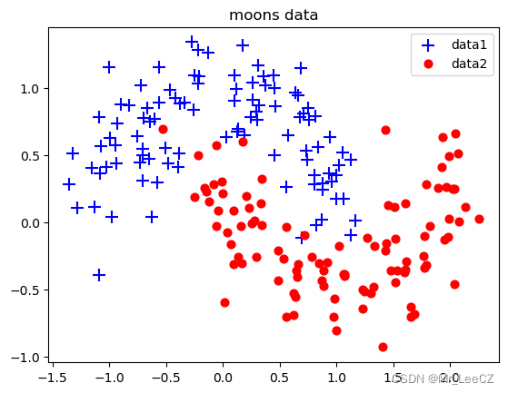
X, Y = sklearn. datasets. make_moons (200, noise=0.2) # 生成内组半圆形数据arg = np.squeeze(np.argwhere(Y==0),axis = 1) # 获取第1类数据索引
arg2 = np.squeeze(np.argwhere (Y==1), axis = 1) # 获取第2类数据索引
plt.title("moons data")
plt.scatter(X[arg,0], X[arg, 1], s=100, c='b' , marker='+' , label='data1')
plt.scatter(X[arg2,0], X[arg2, 1], s=40, c='r' ,marker='o' , label= 'data2')
plt.legend()
plt.show()
#继承nn.Module类,构建网络模型
class LogicNet(nn.Module):def __init__(self,inputdim,hiddendim,outputdim):#初始化网络结构super(LogicNet,self).__init__()self.Linear1 = nn.Linear(inputdim,hiddendim) #定义全连接层self.Linear2 = nn.Linear(hiddendim,outputdim)#定义全连接层self.criterion = nn.CrossEntropyLoss() #定义交叉熵函数def forward(self,x): #搭建用两层全连接组成的网络模型x = self.Linear1(x)#将输入数据传入第1层x = torch.tanh(x)#对第一层的结果进行非线性变换x = self.Linear2(x)#再将数据传入第2层
#        print("LogicNet")return xdef predict(self,x):#实现LogicNet类的预测接口#调用自身网络模型,并对结果进行softmax处理,分别得出预测数据属于每一类的概率pred = torch.softmax(self.forward(x),dim=1)return torch.argmax(pred,dim=1)  #返回每组预测概率中最大的索引def getloss(self,x,y): #实现LogicNet类的损失值计算接口y_pred = self.forward(x)loss = self.criterion(y_pred,y)#计算损失值得交叉熵return lossmodel = LogicNet(inputdim=2,hiddendim=3,outputdim=2)
optimizer = torch.optim.Adam(model.parameters(),lr=0.01)
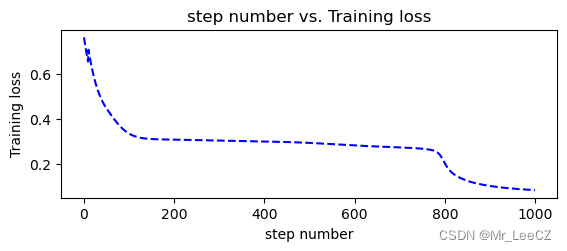
def moving_average(a, w=10):#定义函数计算移动平均损失值if len(a) < w:return a[:]return [val if idx < w else sum(a[(idx-w):idx])/w for idx, val in enumerate(a)]def plot_losses(losses):avgloss= moving_average(losses) #获得损失值的移动平均值plt.figure(1)plt.subplot(211)plt.plot(range(len(avgloss)), avgloss, 'b--')plt.xlabel('step number')plt.ylabel('Training loss')plt.title('step number vs. Training loss')plt.show()
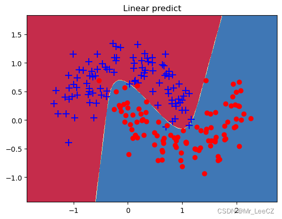
def predict(model,x): #封装支持Numpy的预测接口x = torch.from_numpy(x).type(torch.FloatTensor)ans = model.predict(x)return ans.numpy()def plot_decision_boundary(pred_func,X,Y):#在直角坐标系中可视化模型能力#计算取值范围x_min, x_max = X[:, 0].min() - .5, X[:, 0].max() + .5y_min, y_max = X[:, 1].min() - .5, X[:, 1].max() + .5h = 0.01#在坐标系中采用数据,生成网格矩阵,用于输入模型xx,yy=np.meshgrid(np.arange(x_min, x_max, h), np.arange(y_min, y_max, h))#将数据输入并进行预测Z = pred_func(np.c_[xx.ravel(), yy.ravel()])Z = Z.reshape(xx.shape)#将预测的结果可视化plt.contourf(xx, yy, Z, cmap=plt.cm.Spectral)plt.title("Linear predict")arg = np.squeeze(np.argwhere(Y==0),axis = 1)arg2 = np.squeeze(np.argwhere(Y==1),axis = 1)plt.scatter(X[arg,0], X[arg,1], s=100,c='b',marker='+')plt.scatter(X[arg2,0], X[arg2,1],s=40, c='r',marker='o')plt.show()
if __name__ == '__main__':xt = torch.from_numpy(X).type(torch.FloatTensor)yt = torch.from_numpy(Y).type(torch.LongTensor)epochs = 1000losses = []for i in range(epochs):loss = model.getloss(xt,yt)losses.append(loss.item())optimizer.zero_grad()loss.backward()optimizer.step()plot_losses(losses)print(accuracy_score(model.predict(xt),yt))plot_decision_boundary(lambda x: predict(model,x), xt.numpy(), yt.numpy())
0.98
2. 泰坦尼克号数据分类
2.1 数据的准备工作
计算模块和数据的准备
import os
import numpy as np
import pandas as pd
from scipy import statsimport torch
import torch.nn as nn
import torch.nn.functional as Ftitanic_data = pd.read_csv("titanic3.csv")
print(titanic_data.columns )
print('\n',titanic_data.dtypes)
Index([‘pclass’, ‘survived’, ‘name’, ‘sex’, ‘age’, ‘sibsp’, ‘parch’, ‘ticket’,
‘fare’, ‘cabin’, ‘embarked’, ‘boat’, ‘body’, ‘home.dest’],
dtype=‘object’)
------------
pclass int64
survived int64
name object
sex object
age float64
sibsp int64
parch int64
ticket object
fare float64
cabin object
embarked object
boat object
body float64
home.dest object
dtype: object
对哑变量的处理
#用哑变量将指定字段转成one-hot
titanic_data = pd.concat([titanic_data,pd.get_dummies(titanic_data['sex']),pd.get_dummies(titanic_data['embarked'],prefix="embark"),pd.get_dummies(titanic_data['pclass'],prefix="class")], axis=1)print(titanic_data.columns )
print(titanic_data['sex'])
print(titanic_data['female'])
Index([‘pclass’, ‘survived’, ‘name’, ‘sex’, ‘age’, ‘sibsp’, ‘parch’, ‘ticket’,
‘fare’, ‘cabin’, ‘embarked’, ‘boat’, ‘body’, ‘home.dest’, ‘female’,
‘male’, ‘embark_C’, ‘embark_Q’, ‘embark_S’, ‘class_1’, ‘class_2’,
‘class_3’],
dtype=‘object’)
0 female
1 male
2 female
3 male
4 female
…
1304 female
1305 female
1306 male
1307 male
1308 male
Name: sex, Length: 1309, dtype: object
0 1
1 0
2 1
3 0
4 1
…
1304 1
1305 1
1306 0
1307 0
1308 0
Name: female, Length: 1309, dtype: uint8
对缺失值的处理
#处理None值
titanic_data["age"] = titanic_data["age"].fillna(titanic_data["age"].mean())
titanic_data["fare"] = titanic_data["fare"].fillna(titanic_data["fare"].mean())#乘客票价#删去无用的列
titanic_data = titanic_data.drop(['name','ticket','cabin','boat','body','home.dest','sex','embarked','pclass'], axis=1)
print(titanic_data.columns)
Index([‘survived’, ‘age’, ‘sibsp’, ‘parch’, ‘fare’, ‘female’, ‘male’,
‘embark_C’, ‘embark_Q’, ‘embark_S’, ‘class_1’, ‘class_2’, ‘class_3’],
dtype=‘object’)
划分训练集和测试集
#分离样本和标签
labels = titanic_data["survived"].to_numpy()titanic_data = titanic_data.drop(['survived'], axis=1)
data = titanic_data.to_numpy()#样本的属性名称
feature_names = list(titanic_data.columns)#将样本分为训练和测试两部分
np.random.seed(10)#设置种子,保证每次运行所分的样本一致
train_indices = np.random.choice(len(labels), int(0.7*len(labels)), replace=False)
test_indices = list(set(range(len(labels))) - set(train_indices))
train_features = data[train_indices]
train_labels = labels[train_indices]
test_features = data[test_indices]
test_labels = labels[test_indices]
len(test_labels)#393
2.2 全连接网络的搭建
搭建全连接网络
torch.manual_seed(0)  #设置随机种子class ThreelinearModel(nn.Module):def __init__(self):super().__init__()self.linear1 = nn.Linear(12, 12)self.mish1 = Mish()self.linear2 = nn.Linear(12, 8)self.mish2 = Mish()self.linear3 = nn.Linear(8, 2)self.softmax = nn.Softmax(dim=1)self.criterion = nn.CrossEntropyLoss() #定义交叉熵函数def forward(self, x): #定义一个全连接网络lin1_out = self.linear1(x)out1 = self.mish1(lin1_out)out2 = self.mish2(self.linear2(out1))return self.softmax(self.linear3(out2))def getloss(self,x,y): #实现LogicNet类的损失值计算接口y_pred = self.forward(x)loss = self.criterion(y_pred,y)#计算损失值得交叉熵return lossclass Mish(nn.Module):#Mish激活函数def __init__(self):super().__init__()print("Mish activation loaded...")def forward(self,x):x = x * (torch.tanh(F.softplus(x)))return xnet = ThreelinearModel()
optimizer = torch.optim.Adam(net.parameters(), lr=0.04)
训练网络
num_epochs = 200input_tensor = torch.from_numpy(train_features).type(torch.FloatTensor)
label_tensor = torch.from_numpy(train_labels)losses = []#定义列表,用于接收每一步的损失值
for epoch in range(num_epochs): loss = net.getloss(input_tensor,label_tensor)losses.append(loss.item())optimizer.zero_grad()#清空之前的梯度loss.backward()#反向传播损失值optimizer.step()#更新参数if epoch % 20 == 0:print ('Epoch {}/{} => Loss: {:.2f}'.format(epoch+1, num_epochs, loss.item()))#os.makedirs('models', exist_ok=True)
#torch.save(net.state_dict(), 'models/titanic_model.pt')
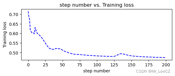
Epoch 1/200 => Loss: 0.72
Epoch 21/200 => Loss: 0.55
Epoch 41/200 => Loss: 0.52
Epoch 61/200 => Loss: 0.49
Epoch 81/200 => Loss: 0.49
Epoch 101/200 => Loss: 0.48
Epoch 121/200 => Loss: 0.48
Epoch 141/200 => Loss: 0.48
Epoch 161/200 => Loss: 0.48
Epoch 181/200 => Loss: 0.48
2.3 结果的可视化
可视化函数
import matplotlib.pyplot as pltdef moving_average(a, w=10):#定义函数计算移动平均损失值if len(a) < w:return a[:]return [val if idx < w else sum(a[(idx-w):idx])/w for idx, val in enumerate(a)]def plot_losses(losses):avgloss= moving_average(losses) #获得损失值的移动平均值plt.figure(1)plt.subplot(211)plt.plot(range(len(avgloss)), avgloss, 'b--')plt.xlabel('step number')plt.ylabel('Training loss')plt.title('step number vs. Training loss')plt.show()
调用可视化函数作图
plot_losses(losses)#输出训练结果
out_probs = net(input_tensor).detach().numpy()
out_classes = np.argmax(out_probs, axis=1)
print("Train Accuracy:", sum(out_classes == train_labels) / len(train_labels))#测试模型
test_input_tensor = torch.from_numpy(test_features).type(torch.FloatTensor)
out_probs = net(test_input_tensor).detach().numpy()
out_classes = np.argmax(out_probs, axis=1)
print("Test Accuracy:", sum(out_classes == test_labels) / len(test_labels))
Train Accuracy: 0.8384279475982532
Test Accuracy: 0.806615776081425