chapter 3 Free electrons in solid - 3.1 自由电子模型
3.1 自由电子模型 Free electron model
研究晶体中的电子:
- 自由电子理论:不考虑离子实
- 能带理论:考虑离子实(周期性势场)的作用
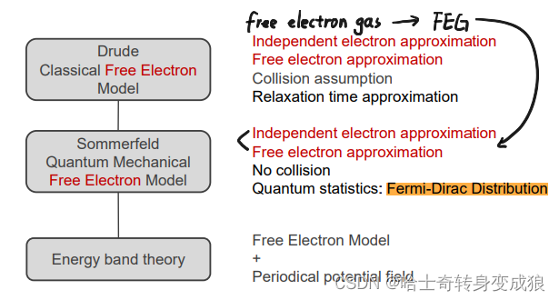
3.1.1 德鲁德模型 Drude Model - Classical Free Electron Model
(1)德鲁德模型
德鲁德模型:价电子游离于特定原子周围,弥散于整个晶体中,形成“自由电子气”。
The Drude model of electrical conduction was proposed in 1900 by Paul Drude to explain the transport properties of electrons in materials (especially metals). The model, which is an application of kinetic theory, assumes that the microscopic behavior of electrons in a solid may be treated classically and looks much like a pinball machine, with a sea of constantly jittering electrons bouncing and re-bouncing off heavier, relatively immobile positive ions.
Assumption of the electron gas:
- 独立电子近似 Independent electron approximation: No electrostatic interaction and collision among free electrons(自由电子之间没有相互作用和碰撞)
- 自由电子近似 Free electron approximation: No electrostatic interaction between free electrons and ions(电子和离子实之间只有碰撞,没有静电相互作用)
- 碰撞假设 Collision assumption: Velocity of electrons after collision with ions only concerns with temperature, but not the velocity before collision(电子和离子实的碰撞是瞬时的,碰撞后的速度仅与温度有关)
- 弛豫时间近似 Relaxation time approximation: Relaxation time τ is independent with the position and velocity of electrons(弛豫时间即同一粒子两次碰撞的时间间隔,它仅依赖于晶体结构)
在德鲁德模型中,存在电场时,电子每两次碰撞之间都会获得电场加速,从而形成漂移速度 v d v_d vd,且漂移速度远小于电子热运动的速度 v d ≪ v R M S = 3 k B T m v_d \ll v_{RMS} = \sqrt{\frac{3k_BT}{m}} vd≪vRMS=m3kBT
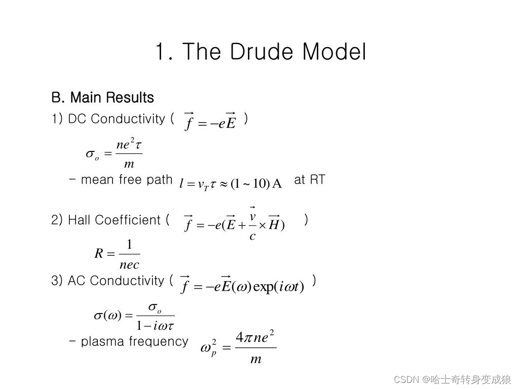
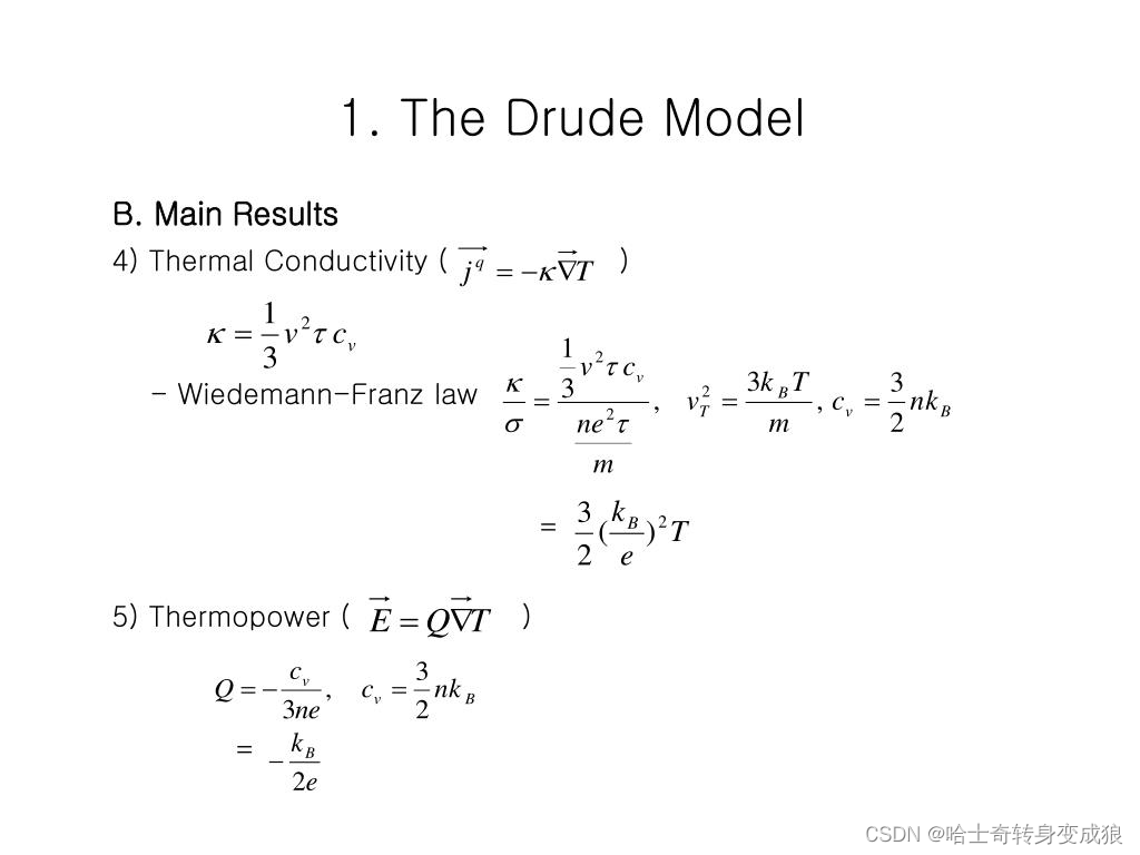
利用德鲁德模型能够成功解释:
- 欧姆定律
- Wiedemann-Franz ratio comes out close to right for most materials
- Many other transport properties predicted correctly
(2) failure of Drude Model
德鲁德模型存在的问题:
- 电子比热 Specific Heat of electrons
- 电导率与温度的关系 Temperature dependence of σ
- Wiedemann-Franz ratio
- The Seebeck/Peltier coefficient come out wrong by a factor of 100.
Despite the shortcomings of Drude theory, it nonetheless was the only theory of metallic conductivity for a quarter of a century (until the Sommerfeld theory improved it), and it remains quite useful today.
3.1.2 索末菲模型 Sommerfeld Model - Quantum Mechanical Free Electron Model
索末菲保留了德鲁德的自由电子气假设(前两个),但是索末菲去除了“碰撞”的概念,引入量子统计的理论(费米-狄拉克分布 Fermi-Dirac Distribution)。
(1)势阱 potential well
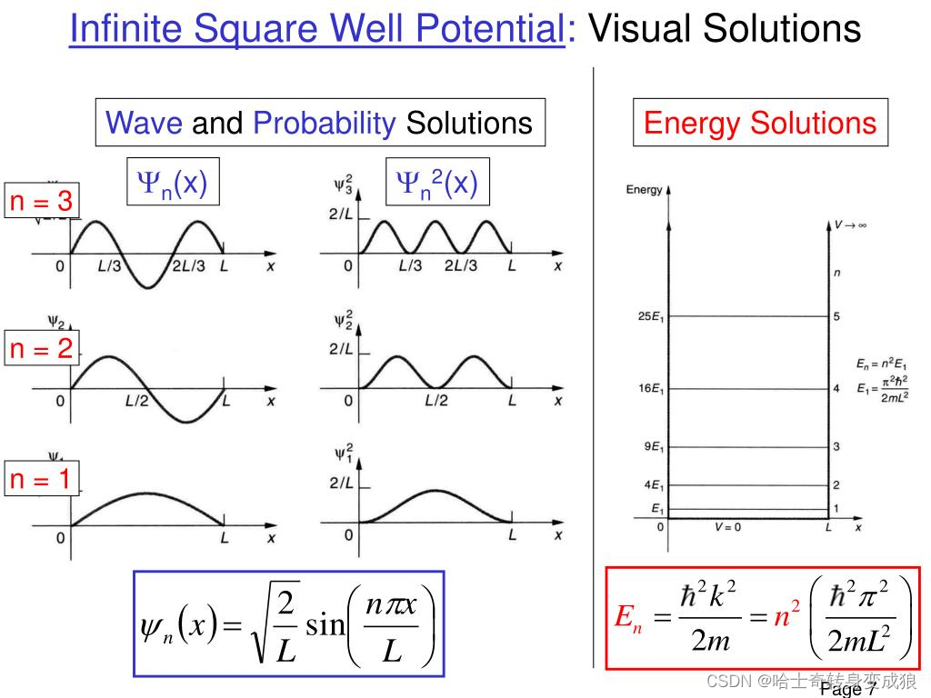
1D Infinite Potential Well
( − ℏ 2 2 m d 2 d x 2 + U ( x ) ) ψ ( x ) = E ψ ( x ) \left( -\frac{\hbar^2}{2m} \frac{d^2}{dx^2} + U(x) \right ) \psi (x) = E \psi(x) (−2mℏ2dx2d2+U(x))ψ(x)=Eψ(x)
k = n π L , n = 1 , 2 , 3 , … k = n \frac{\pi}{L}, \ \ n=1,2,3,\dots k=nLπ, n=1,2,3,…
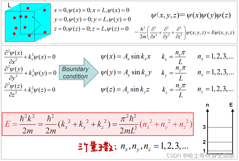
3D Infinite Potential Well
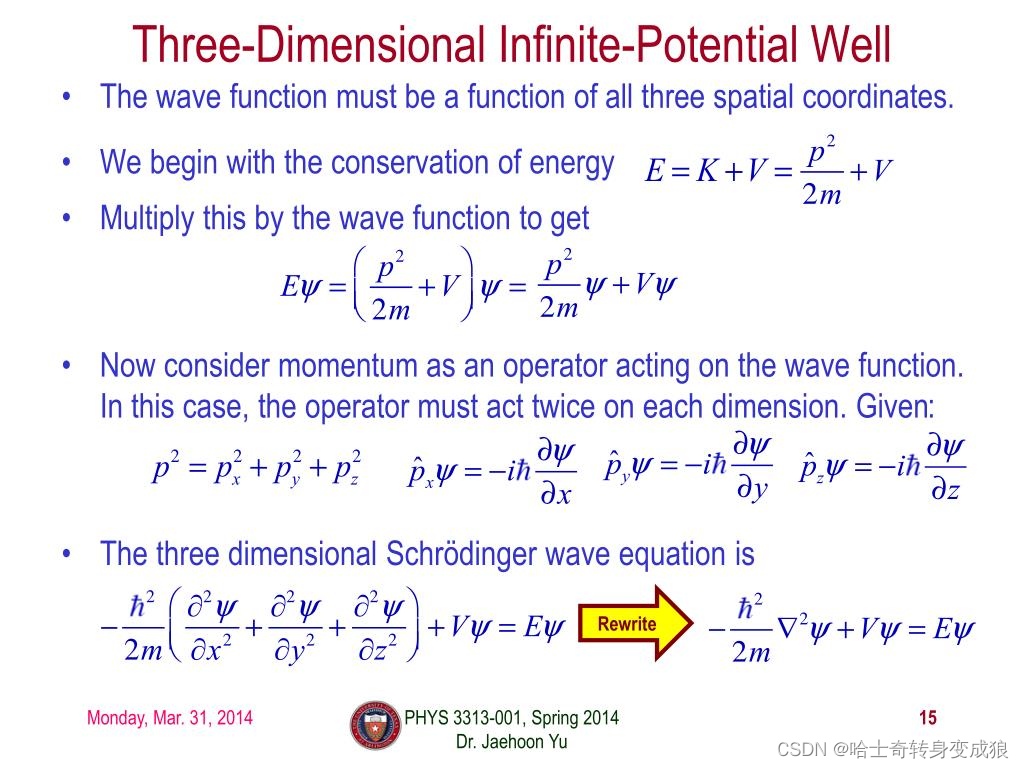
− ℏ 2 2 m ( ∂ 2 ∂ x 2 + ∂ 2 ∂ y 2 + ∂ 2 ∂ z 2 ) ψ ( x , y , z ) = E ψ ( x , y , z ) -\frac{\hbar ^2}{2m}\left( \frac{\partial^2}{\partial x^2} + \frac{\partial^2}{\partial y^2} + \frac{\partial^2}{\partial z^2} \right) \psi(x,y,z) = E \psi (x,y,z) −2mℏ2(∂x2∂2+∂y2∂2+∂z2∂2)ψ(x,y,z)=Eψ(x,y,z)
ψ ( x , y , z ) = ψ ( x ) ψ ( y ) ψ ( z ) \psi(x,y,z) = \psi(x) \psi(y) \psi(z) ψ(x,y,z)=ψ(x)ψ(y)ψ(z)
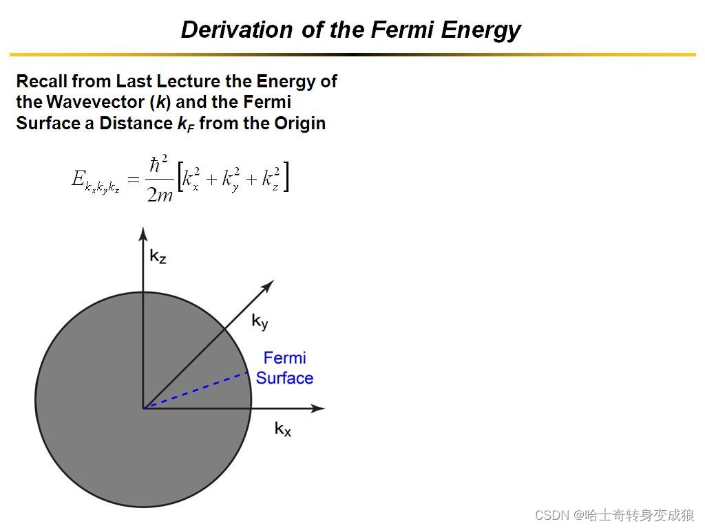
∵ E = ℏ 2 k 2 2 m , k ⃗ = k x i ⃗ + k y j ⃗ + k z l ⃗ \because E = \frac{\hbar ^2 k^2}{2m}, \ \ \vec k = k_x \vec i + k_y \vec j + k_z \vec l ∵E=2mℏ2k2, k=kxi+kyj+kzl
∴ E = ℏ 2 2 m ( k x 2 + k y 2 + k z 2 ) \therefore E = \frac{\hbar^2}{2m} (k_x^2 + k_y^2 + k_z^2) ∴E=2mℏ2(kx2+ky2+kz2)
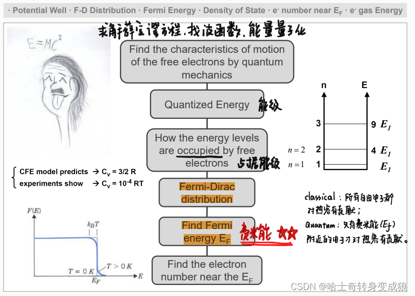
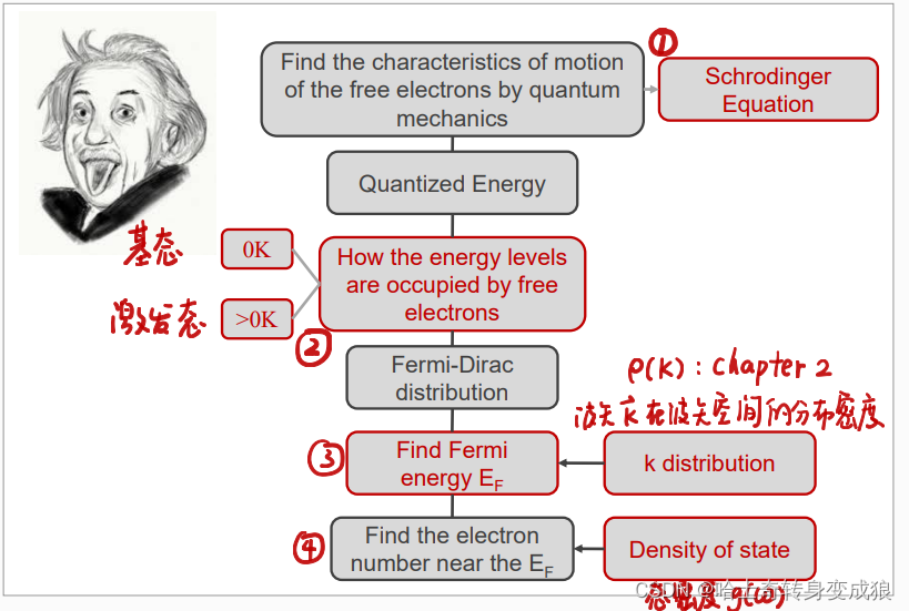
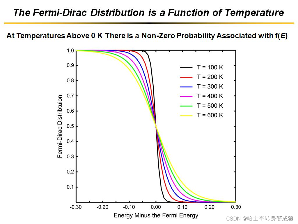
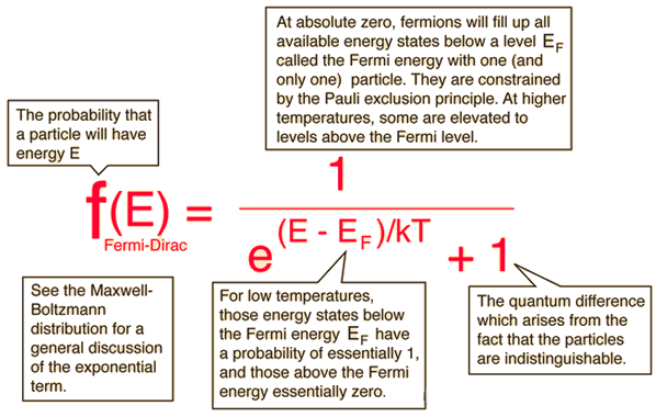
(2)费米-狄拉克分布与费米能 Fermi-Dirac distribution & Fermi Energy
F l = α l ω l = 1 e ( α + β E l ) + 1 = 1 e ( E l − μ ) / k B T + 1 = 1 e ( E l − E F ) / k B T + 1 F_l = \frac{\alpha _l}{\omega _ l} = \frac{1}{e^{(\alpha + \beta E_l)} + 1} = \frac{1}{e^{(E_l - \mu)/k_B T} + 1} = \frac{1}{e^{(E_l - E_F)/k_B T} + 1} Fl=ωlαl=e(α+βEl)+11=e(El−μ)/kBT+11=e(El−EF)/kBT+11
a. Classical theory of Occupancy Condition at T=0K
- 电子能量可以相同,不同电子可以占据同一能级,即不同电子具有相同的量子态。
- 电子分布满足Maxwell-Boltzmann分布。
- 一个系统的温度反应了系统内粒子运动的动能,T=0,所有电子静止不动。 1 2 m v ˉ 2 = 3 2 k B T , ∴ T = 0 K , v = 0 \frac{1}{2} m \bar v^2 = \frac{3}{2}k_B T,\ \ \ \therefore T=0K,\ v=0 21mvˉ2=23kBT, ∴T=0K, v=0
b. Quantum mechanically of Occupancy Condition at T=0K
Pauli’s Exclusion Principle:两个费米子不能处于同一量子态。
考虑自旋,一个能级对应有f组量子数,即有f重简并,这一个能级可以放2f个电子。
费米能级:在绝对零度时,一个费米子具有的最高能量。
The Fermi energy : the highest energy a fermion can take at absolute zero temperature.
假想把所有的费米子从量子态上移开,之后再把这些费米子按照一定的规则填充在各个可供占据的能量态上,并且这种填充过程中每个费米子都占据最低的可供占据的量子态。最后一个费米子占据的量子态即可粗略地认为是费米能级。
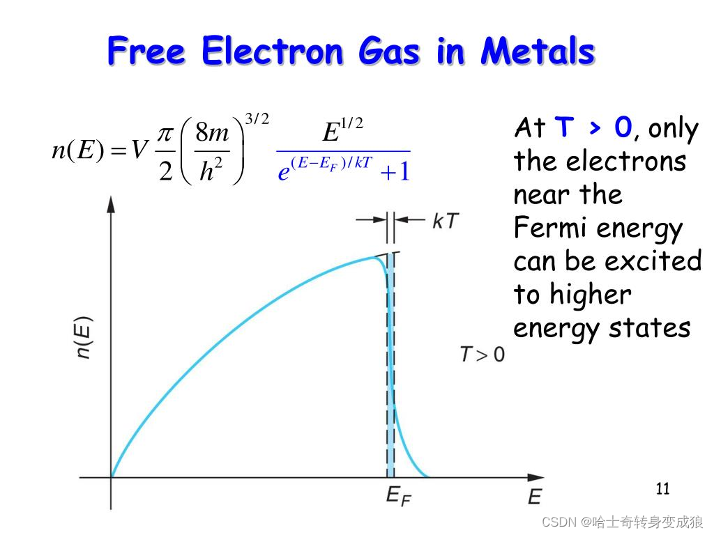
c. Quantum mechanically of Occupancy Condition at T>0K
CFE model predicts: C V = 3 2 R C_V=\frac{3}{2}R CV=23R
experiments show: C V = 1 0 − 4 R T C_V = 10^{-4} RT CV=10−4RT
经典自由电子模型认为,所有电子都会对热容有贡献;量子力学认为,只有费米能级附近的电子才有可能脱离原子,具有导电特性,因为高能级被占据导致低能级电子无法跃迁。
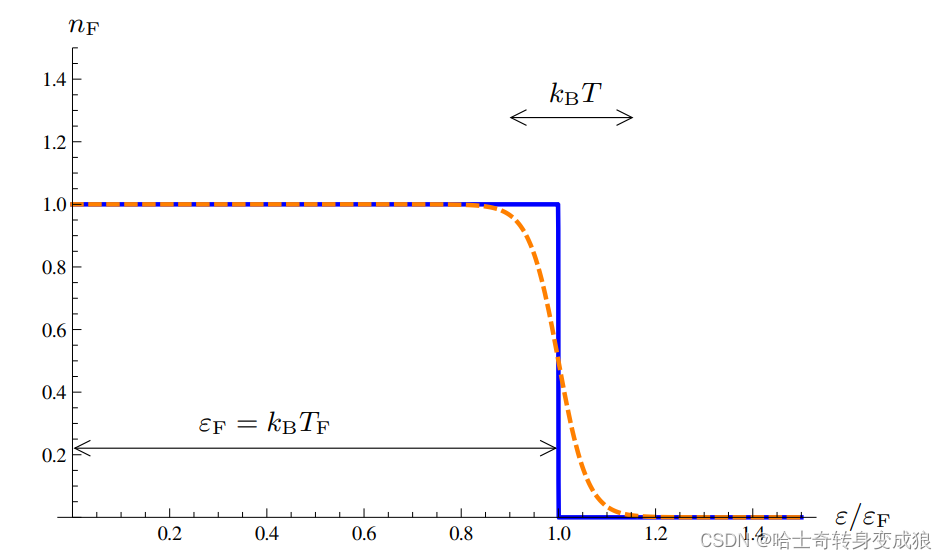
The Fermi–Dirac distribution at zero temperature (solid line) constitutes a step function. For T > 0 (dashed line), broadening appears in a region of width k B T k_B T kBT around the Fermi edge located at ε = ε F = k B T F . ε = ε_F = k_B T_F. ε=εF=kBTF. If the distance of the edge from the origin is much larger than the area of broadening, the distribution function still displays the characteristic step-like behavior. Clearly, this picture is valid for the dimensionless parameter T / T F T/T_F T/TF being small.
(3)计算0K时的费米能 Fermi Energy at T=0K
视频讲解:费米能和态密度
KaTeX parse error: Undefined control sequence: \k at position 20: …= \frac{(\hbar \̲k̲_F)^2}{2m}
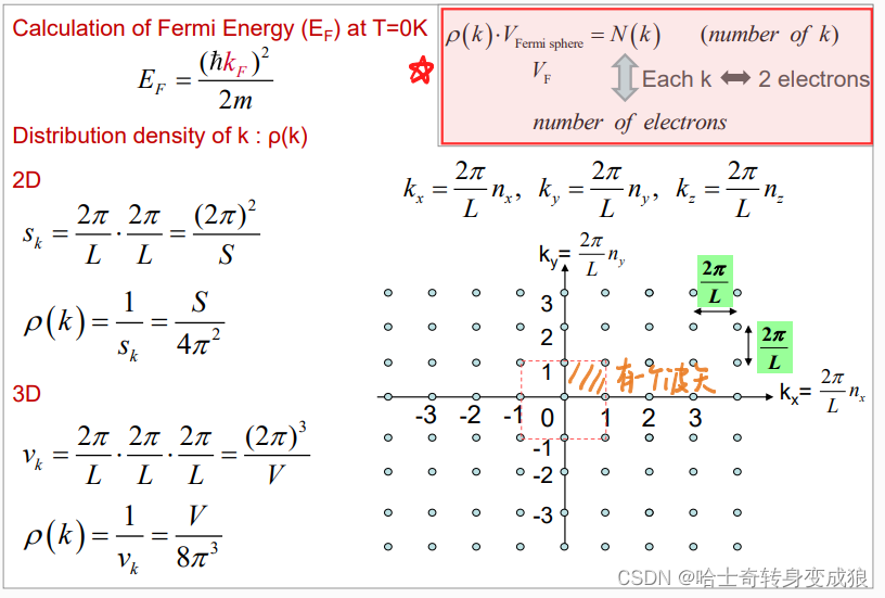
n u m b e r o f k : V F ⋅ ρ ( k ) = ( 4 π k F 3 3 ) ( V 8 π 3 ) = k F 3 6 π 2 V number \ of \ k: \ V_F \cdot \rho(k) = \left(\frac{4\pi k_F^3}{3} \right) \left( \frac{V}{8\pi^3} \right) = \frac{k_F^3}{6\pi^2}V number of k: VF⋅ρ(k)=(34πkF3)(8π3V)=6π2kF3V
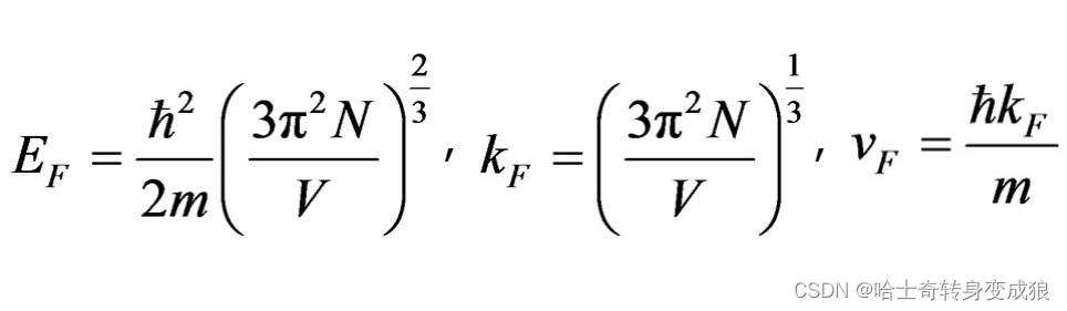
where N is the total number of electrons, n=N/V is the total number of electrons per unit volume in the alloy, m is the effective mass, ħ is the reduced Plank’s constant
Fermi temperature T F T_F TF: T F = E F k B T_F = \frac{E_F}{k_B} TF=kBEF
费米能级对应的费米球的半径是费米半径,对应的费米面是电子占据能级和不占据的分界面。
Fermi sphere: 费米面
Fermi wave vector k F k_F kF: 费米波矢 the radius of the Fermi sphere
At T=0K, inside Fermi sphere, all orbits are occupied; outside Fermi sphere, all orbits are empty.
(4)态密度 density of state
态密度:单位能量间隔电子能态(量子态或者轨道)的数量。
DOS: the number of electronic energy states (orbits) per unit energy.
g ( E ) = d Z d E g(E) = \frac{dZ}{dE} g(E)=dEdZ
In crystal dynamics, the density of states g(ω) is defined as the number of oscillators (or k) per unit frequency interval.
Each k state represents two possible electron states: (考虑自旋,一个k态对应两个可能的电子能量态)
one for spin up, the other for spin down, thus the total number of electronic states in a sphere of diameter k is: Z ( E ) = 2 ⋅ ρ ( k ) ⋅ 4 3 π k 3 = V k 3 3 π 2 Z(E) = 2\cdot \rho(\mathbf{k}) \cdot \frac{4}{3} \pi k^3 = \frac{Vk^3}{3\pi^2} Z(E)=2⋅ρ(k)⋅34πk3=3π2Vk3
consider: E = ℏ 2 k 2 2 m E = \frac{\hbar ^2 k^2}{2m} E=2mℏ2k2
g ( E ) = d Z d E = d Z d k ⋅ d k d E g(E) = \frac{dZ}{dE} = \frac{dZ}{dk}\cdot \frac{dk}{dE} g(E)=dEdZ=dkdZ⋅dEdk
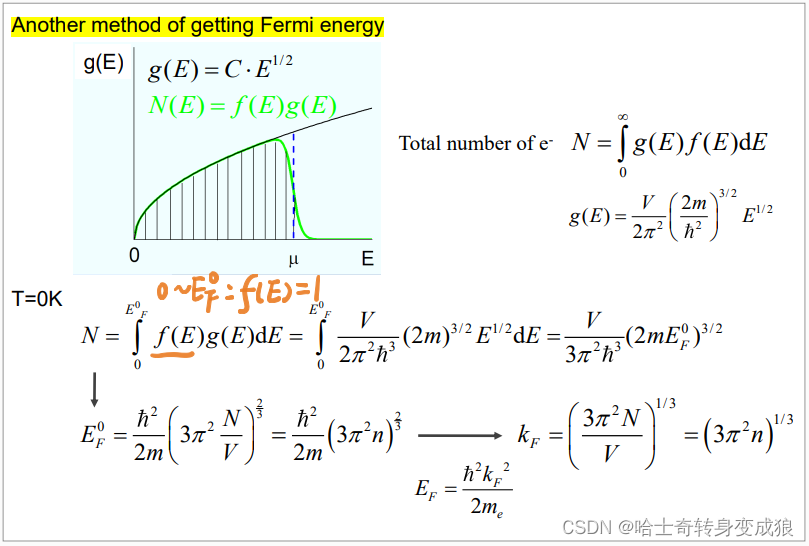
∴ g ( E ) = V 2 π 2 ( 2 m ℏ 2 ) 3 / 2 \therefore g(E) = \frac{V}{2\pi^2} \left( \frac{2m}{\hbar^2}\right)^{3/2} ∴g(E)=2π2V(ℏ22m)3/2
g ( E ) = C ⋅ E 1 / 2 g(E) = C\cdot E^{1/2} g(E)=C⋅E1/2
{ 1 D : g ( E ) = C ⋅ E − 1 / 2 2 D : g ( E ) = m S π ℏ 2 3 D : g ( E ) = C ⋅ E − 1 / 2 \begin{cases} 1D: g(E) = C\cdot E^{-1/2} \\ 2D: g(E) = \frac{mS}{\pi \hbar^2} \\ 3D: g(E) = C\cdot E^{-1/2} \end{cases} ⎩ ⎨ ⎧1D:g(E)=C⋅E−1/22D:g(E)=πℏ2mS3D:g(E)=C⋅E−1/2
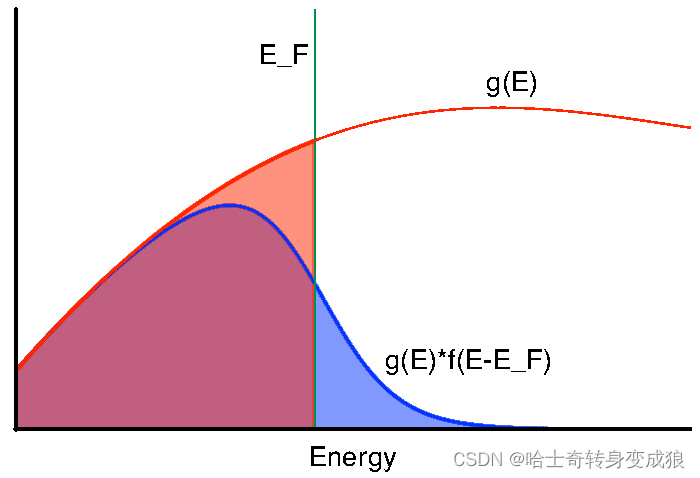
(5)费米能级附近的电子数量 e- number near E F E_F EF
DOS g(E): the number of electronic energy states (orbits) per unit energy.
f(E): probability that an electronic energy state be occupied.
N(E):电子能量分布函数 Electron energy distribution function
N(E)dE = number of e- with energies between E and E+dE
g(E)f(E)dE = number of e- with energies between E and E+dE
N ( E ) = g ( E ) f ( E ) N(E) = g(E)f(E) N(E)=g(E)f(E)
total number of e-: N = ∈ 0 ∞ g ( E ) f ( E ) d E N = \in_0^{\infty} g(E)f(E)dE N=∈0∞g(E)f(E)dE
下面这个方法很合适:
(6)电子气能量 e- gas energy
Total energy for electron gas:
T=0K :
E t = ∫ E d N = ∫ E ⋅ g ( E ) f ( E ) d E = ∫ 0 E F 0 C ⋅ E 1 / 2 d E = ∫ 0 E F 0 C E 3 / 2 d E = 2 C 5 ( E F 0 ) 5 / 2 E_t = \int EdN = \int E\cdot g(E)f(E)dE = \int_0^{E_F^0} C\cdot E^{1/2} dE = \int_0^{E_F^0} CE^{3/2}dE = \frac{2C}{5}(E_F^0)^{5/2} Et=∫EdN=∫E⋅g(E)f(E)dE=∫0EF0C⋅E1/2dE=∫0EF0CE3/2dE=52C(EF0)5/2
Average energy for free electrons:
E ˉ = E t N = 3 5 E F 0 \bar E = \frac{E_t}{N} = \frac{3}{5}E_F^0 Eˉ=NEt=53EF0
E t = 3 5 N E F 0 E_t = \frac{3}{5}NE_F^0 Et=53NEF0
At T=0K,the average energy of a free electron is 60% of the Femi energy.
T>0K :
E t = ∫ E ⋅ g ( E ) f ( E ) d E = C ∫ 0 ∞ E 3 / 2 1 e ( E − E F ) / k B T + 1 = … = 3 5 N E F 0 [ 1 + 5 12 π 2 ( k B T E F 0 ) 2 ] \begin{align} E_t &=\int E\cdot g(E)f(E)dE \\ &= C \int_0^{\infty} E^{3/2} \frac{1}{e^{(E-E_F)/k_B T}+1} \\ & =\dots \\ &= \frac{3}{5}N E_F^0 [1+ \frac{5}{12}\pi^2 (\frac{k_B T}{E_F^0})^2] \end{align} Et=∫E⋅g(E)f(E)dE=C∫0∞E3/2e(E−EF)/kBT+11=…=53NEF0[1+125π2(EF0kBT)2]
第一项是零点能,第二项由于分母的费米能很大所以可以忽略不计。
温度升高,热容涨幅不明显
E F = E F 0 [ 1 − 1 12 π 2 ( k B T E F 0 ) 2 ] = E F 0 [ 1 − π 2 12 ( T T F ) 2 ] ≈ E F 0 E_F = E_F^0 \left[1- \frac{1}{12}\pi^2 (\frac{k_B T}{E_F^0})^2 \right] = E_F^0 \left[1-\frac{\pi^2}{12}\left( \frac{T}{T_F}\right)^2 \right] \approx E_F^0 EF=EF0[1−121π2(EF0kBT)2]=EF0[1−12π2(TFT)2]≈EF0