econml双机器学习实现连续干预和预测
连续干预
在这个示例中,我们使用LinearDML模型,使用随机森林回归模型来估计因果效应。我们首先模拟数据,然后模型,并使用方法来effect创建不同干预值下的效应(Conditional Average Treatment Effect,CATE)。
请注意,实际情况中的数据可能更加复杂,您可能需要根据您的数据和问题来适当选择的模型和参数。此示例仅供参考,您可以根据需要进行修改和扩展。
import numpy as np
from econml.dml import LinearDML# 生成示例数据
np.random.seed(123)
n_samples = 1000
n_features = 5
X = np.random.normal(size=(n_samples, n_features))
T = np.random.uniform(low=0, high=1, size=n_samples) # 连续干预变量
y = 2 * X[:, 0] + 0.5 * X[:, 1] + 3 * T + np.random.normal(size=n_samples)# 初始化 LinearDML 模型
est = LinearDML(model_y='auto', model_t='auto', random_state=123)# 拟合模型
est.fit(y, T, X=X)# 给定特征和连续干预值,计算干预效应
X_pred = np.random.normal(size=(10, n_features)) # 假设有新的数据点 X_pred
T_pred0 = np.array([0]*10) # 指定的连续干预值
T_pred11 = np.array([0.2, 0.4, 0.6, 0.8, 1.0, 0.3, 0.5, 0.7, 0.9, 0.1]) # 指定的连续干预值
T_pred1 = np.array([0.2]*10) # 指定的连续干预值
T_pred2 = np.array([0.4]*10) # 指定的连续干预值
T_pred3 = np.array([0.6]*10) # 指定的连续干预值
T_pred4 = np.array([0.8]*10) # 指定的连续干预值# 计算连续干预效应
effect_pred = est.effect(X=X_pred, T0=T_pred0, T1=T_pred11)print("预测的连续干预效应:", effect_pred)# 计算连续干预效应
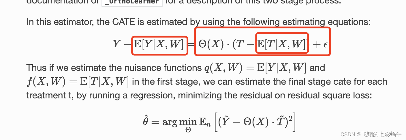
effect_pred = est.effect(X=X_pred, T0=T_pred0, T1=T_pred1)print("预测的连续干预效应:", effect_pred)The R Learner is an approach for estimating flexible non-parametric models of conditional average treatment effects in the setting with no unobserved confounders. The method is based on the idea of Neyman orthogonality and estimates a CATE whose mean squared error is robust to the estimation errors of auxiliary submodels that also need to be estimated from data:
the outcome or regression model
the treatment or propensity or policy or logging policy model
使用随机实验数据进行双重机器学习(DML)训练可能会在某些情况下获得更好的效果,但并不是绝对的规律。DML方法的性能取决于多个因素,包括数据质量、特征选择、模型选择和调参等。
使用随机实验数据进行训练的优势在于,实验数据通常可以更好地控制混淆因素,从而更准确地估计因果效应。如果实验设计得当,并且随机化合理,那么通过DML训练的模型可以更好地捕捉因果关系,从而获得更准确的效应估计。
然而,即使使用随机实验数据,DML方法仍然需要考虑一些因素,例如样本大小、特征的选择和处理、模型的选择和调参等。在实际应用中,没有一种方法可以适用于所有情况。有时,随机实验数据可能会受到实验设计的限制,或者数据质量可能不足以获得准确的效应估计。
因此,使用随机实验数据进行DML训练可能会在某些情况下获得更好的效果,但并不是绝对的规律。在应用DML方法时,仍然需要根据实际情况进行数据分析、模型选择和验证,以确保获得准确和可靠的因果效应估计。
连续干预/label01
import numpy as np
from econml.dml import LinearDML
import scipy# 生成示例数据
np.random.seed(123)
n_samples = 1000
n_features = 5
X = np.random.normal(size=(n_samples, n_features))
T = np.random.uniform(low=0, high=1, size=n_samples)  # 连续干预变量
#y = 2 * X[:, 0] + 0.5 * X[:, 1] + 3 * T + np.random.normal(size=n_samples)
y = np.random.binomial(1, scipy.special.expit(X[:, 0]))# 初始化 LinearDML 模型
est = LinearDML(model_y='auto', model_t='auto', random_state=123)# 拟合模型
est.fit(y, T, X=X)# 给定特征和连续干预值,计算干预效应
X_pred = np.random.normal(size=(10, n_features))  # 假设有新的数据点 X_pred
T_pred0 = np.array([0]*10)  # 指定的连续干预值
T_pred11 = np.array([0.2, 0.4, 0.6, 0.8, 1.0, 0.3, 0.5, 0.7, 0.9, 0.1])  # 指定的连续干预值
T_pred1 = np.array([0.2]*10)  # 指定的连续干预值
T_pred2 = np.array([0.4]*10)  # 指定的连续干预值
T_pred3 = np.array([0.6]*10)  # 指定的连续干预值
T_pred4 = np.array([0.8]*10)  # 指定的连续干预值# 计算连续干预效应
effect_pred = est.effect(X=X_pred, T0=T_pred0, T1=T_pred11)print("预测的连续干预效应:", effect_pred)
预测的连续干预效应: [-0.00793674 0.00612109 0.03141778 0.00310806 -0.01635394 -0.019054340.06801354 -0.0126543 -0.04603434 0.00821044]
dml原理
Double Machine Learning, DML。
方法:首先通过X预测T,与真实的T作差,得到一个T的残差,然后通过X预测Y,与真实的Y作差,得到一个Y的残差,预测模型可以是任何ML模型,最后基于T的残差和Y的残差进行因果建模。
原理:DML采用了一种残差回归的思想。
优点:原理简单,容易理解。预测阶段可以使用任意ML模型。
缺点: 需要因果效应为线性的假设。
应用场景:适用于连续Treatment且因果效应为线性场景
单调性约束
因果推断的开源包中,有一些可以进行单调性约束的案例。这些案例通常涉及到因果效应的估计,同时加入了单调性约束以确保结果更加合理和可解释。以下是一些开源包以及它们支持单调性约束的案例示例:
-
CausalML(https://causalml.readthedocs.io/):
CausalML 是一个开源的因果推断工具包,支持单调性约束。它提供了一些可以用于处理单调性约束的方法,例如SingleTreatment类。您可以使用该包来在处理因果效应时添加单调性约束。
-
econml(https://econml.azurewebsites.net/):
- econml 也是一个用于因果推断的工具包,支持单调性约束。它提供了一些工具,如
SingleTreePolicyInterpreter和SingleTreeCateInterpreter,用于解释单一决策树的因果效应,并且可以根据用户指定的特征添加单调性约束。
- econml 也是一个用于因果推断的工具包,支持单调性约束。它提供了一些工具,如
SingleTreeCateInterpreter(_SingleTreeInterpreter):"""An interpreter for the effect estimated by a CATE estimatorParameters----------include_model_uncertainty : bool, default FalseWhether to include confidence interval information when building asimplified model of the cate model. If set to True, thencate estimator needs to support the `const_marginal_ate_inference` method.uncertainty_level : double, default 0.05The uncertainty level for the confidence intervals to be constructedand used in the simplified model creation. If value=alphathen a multitask decision tree will be built such that all samplesin a leaf have similar target prediction but also similar alphaconfidence intervals.uncertainty_only_on_leaves : bool, default TrueWhether uncertainty information should be displayed only on leaf nodes.If False, then interpretation can be slightly slower, especially for catemodels that have a computationally expensive inference method.