scikit-plot 使用笔记
scikit-plot是基于sklearn和Matplotlib的库,主要的功能是对训练好的模型进行可视化。
安装:
pip install scikit-plot功能1:评估指标可视化
scikitplot.metrics.plot_confusion_matrix快速展示模型预测结果和标签计算得到的混淆矩阵。

import scikitplot as skpltrf = RandomForestClassifier()rf = rf.fit(X_train, y_train)y_pred = rf.predict(X_test)skplt.metrics.plot_confusion_matrix(y_test, y_pred, normalize=True)plt.show()
scikitplot.metrics.plot_roc快速展示模型预测的每个类别的ROC曲线。

import scikitplot as skplt
nb = GaussianNB()
nb = nb.fit(X_train, y_train)
y_probas = nb.predict_proba(X_test)skplt.metrics.plot_roc(y_test, y_probas)
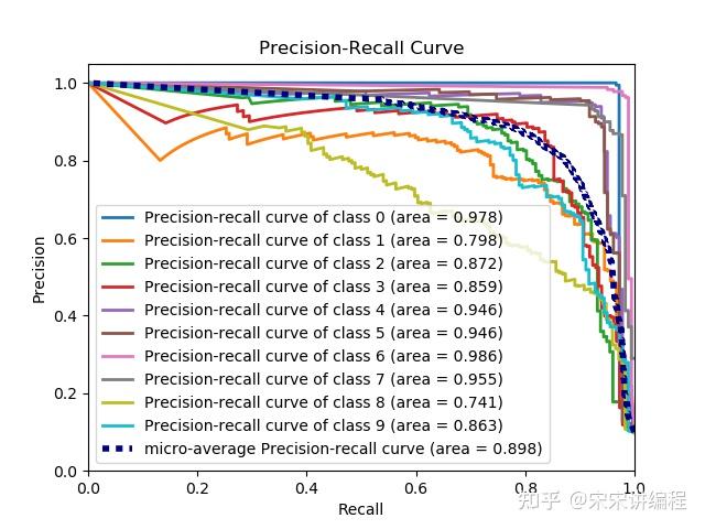
plt.show()scikitplot.metrics.plot_precision_recall从标签和概率生成PR曲线
import scikitplot as skplt
nb = GaussianNB()
nb.fit(X_train, y_train)
y_probas = nb.predict_proba(X_test)skplt.metrics.plot_precision_recall(y_test, y_probas)
plt.show()
scikitplot.metrics.plot_calibration_curve绘制分类器的矫正曲线

import scikitplot as skplt
rf = RandomForestClassifier()
lr = LogisticRegression()
nb = GaussianNB()
svm = LinearSVC()
rf_probas = rf.fit(X_train, y_train).predict_proba(X_test)
lr_probas = lr.fit(X_train, y_train).predict_proba(X_test)
nb_probas = nb.fit(X_train, y_train).predict_proba(X_test)
svm_scores = svm.fit(X_train, y_train).decision_function(X_test)
probas_list = [rf_probas, lr_probas, nb_probas, svm_scores]
clf_names = ['Random Forest', 'Logistic Regression','Gaussian Naive Bayes', 'Support Vector Machine']skplt.metrics.plot_calibration_curve(y_test,probas_list,clf_names)
plt.show()
功能2:模型可视化
scikitplot.estimators.plot_learning_curve生成不同训练样本下的训练和测试学习曲线图
import scikitplot as skplt
rf = RandomForestClassifier()skplt.estimators.plot_learning_curve(rf, X, y)
plt.show()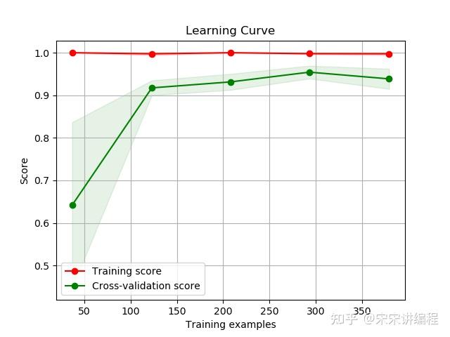
scikitplot.estimators.plot_feature_importances可视化特征重要性。
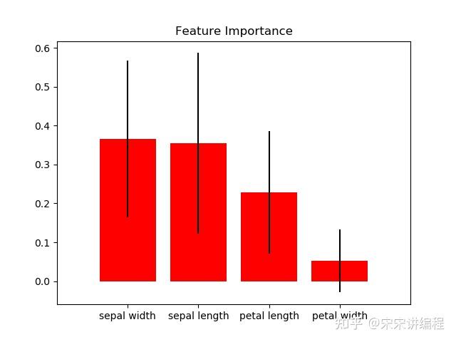
import scikitplot as skplt
rf = RandomForestClassifier()
rf.fit(X, y)skplt.estimators.plot_feature_importances(rf, feature_names=['petal length', 'petal width','sepal length', 'sepal width'])
plt.show()
功能3:聚类可视化
- scikitplot.cluster.plot_elbow_curve展示聚类的肘步图。
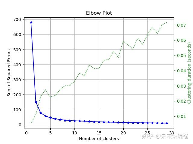
import scikitplot as skplt
kmeans = KMeans(random_state=1)skplt.cluster.plot_elbow_curve(kmeans, cluster_ranges=range(1, 30))
plt.show()
功能4:降维可视化
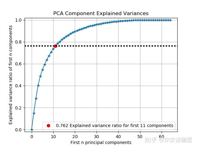
- scikitplot.decomposition.plot_pca_component_variance绘制 PCA 分量的解释方差比。
import scikitplot as skplt
pca = PCA(random_state=1)
pca.fit(X)skplt.decomposition.plot_pca_component_variance(pca)plt.show()
scikitplot.decomposition.plot_pca_2d_projection绘制PCA降维之后的散点图。
import scikitplot as skplt
pca = PCA(random_state=1)
pca.fit(X)skplt.decomposition.plot_pca_2d_projection(pca, X, y)
plt.show()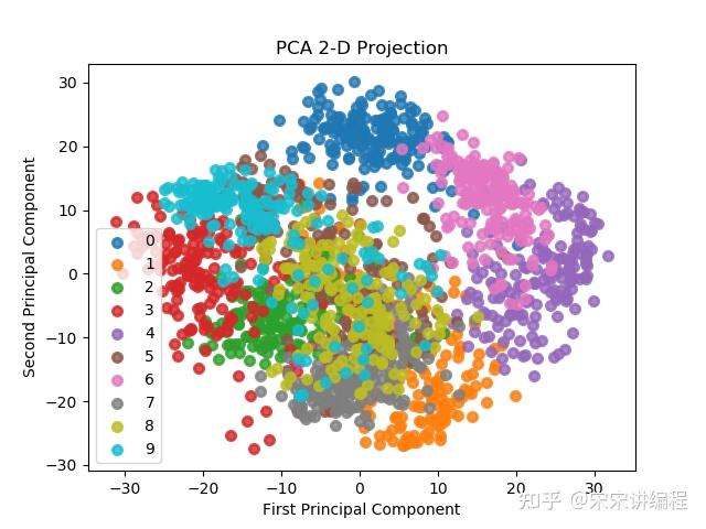
principle components(主成分)是通过线性变换从原始数据中提取出来的新变量。主成分是原始数据的线性组合,通过这种方式,它们能够捕捉到数据中的最大方差。
PCA的目标是将高维数据转换为一组低维的主成分,这些主成分将数据中的方差解释得尽可能好。第一个主成分解释了最大的方差,第二个主成分解释了次大的方差,以此类推。每个主成分都是关于原始特征的线性组合,并且它们之间是正交的(相互之间不相关)。
主成分类似于原始数据的投影,但是它们的排序是如此安排,以便第一个主成分解释了最大的方差,第二个主成分解释了次大的方差,以此类推。这允许我们选择在最小信息损失的情况下保留具有最高方差的主要特征,并减少数据的维度。