当前位置：首页 > news >正文

实数信号的傅里叶级数研究（Matlab代码实现）

news 2025/6/21 19:31:04

💥💥💞💞欢迎来到本博客❤️❤️💥💥

🏆博主优势：🌞🌞🌞博客内容尽量做到思维缜密，逻辑清晰，为了方便读者。

⛳️座右铭：行百里者，半于九十。

📋📋📋本文目录如下：🎁🎁🎁

目录

💥1 概述

📚2 运行结果

🎉3 参考文献

🌈4 Matlab代码实现

💥1 概述

实数信号的傅里叶级数是将实数信号分解为一系列正弦和余弦函数的和。通过研究实数信号的傅里叶级数，我们可以揭示信号的频域特性、谐波成分以及信号的周期性等信息。

以下是实数信号的傅里叶级数研究的步骤：

1. 确定信号的周期：实数信号的傅里叶级数要求信号是周期性的，因此第一步是确定信号的周期。如果信号已知周期，则直接使用已知的周期；如果信号的周期未知，可以通过观察信号的重复性或通过分析信号的特征来估计周期。

2. 计算基频和谐波频率：基频是指信号的周期的倒数，而谐波频率是基频的整数倍。通过计算基频和谐波频率，可以确定傅里叶级数中需要考虑的频率分量。

3. 计算信号的系数：使用傅里叶级数的公式，根据信号的周期和所选的频率分量，计算信号在每个频率分量上的系数。系数表示了每个频率分量对于信号的贡献程度。

4. 重构信号：将计算得到的正弦和余弦函数按照其对应的系数加权求和，可以重构出原始信号的近似，即使用傅里叶级数近似表示原始信号。

5. 分析频域特性和谐波成分：通过观察每个频率分量的系数，可以了解信号在频域上的特性。特别是谐波成分在系数中的存在可以揭示信号中的谐波结构和频率分布情况。

6. 评估和调整：根据计算得到的傅里叶级数近似信号和频域分析结果，评估傅里叶级数的逼近效果，并进行必要的调整和优化。

需要注意的是，实数信号的傅里叶级数研究需要信号是周期性的。对于非周期信号，可以考虑使用傅里叶变换进行频域分析。

总之，实数信号的傅里叶级数研究包括确定信号的周期、计算基频和谐波频率、计算信号的系数、重构信号、分析频域特性和谐波成分等步骤。通过这些步骤，我们可以深入了解信号的频域特性和谐波成分，从而更好地理解和处理实数信号。

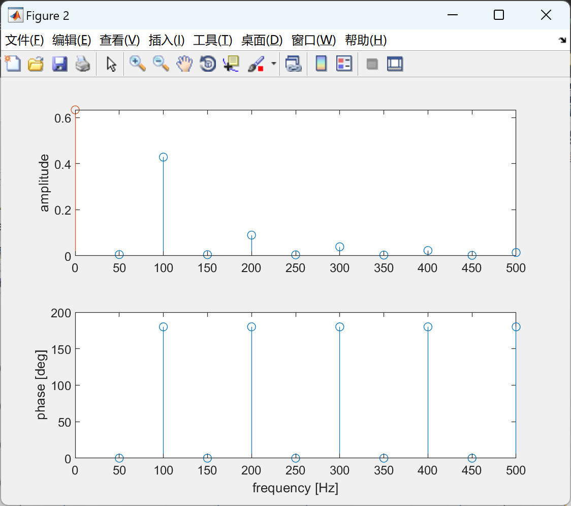
📚2 运行结果

部分代码：

function [ freq,amp,phase,dc ] = fourier_series_real( t,x )
% function [ freq,amp,phase,dc ] = fourier_series_real( t,x )
% Fourier series of real signals.
% Written by Yoash Levron, January 2013.
%
% This function computes the fourier series of a signal x(t).
% the amplitudes of the fourier series have the same dimension
% of the original signal, so this function is useful for immediate
% computation of the actual frequency components, without
% further processing.
%
% for example, x(t) = 2 + 3*cos(2*pi*50*t) will result in
% dc value = 2
% frequencies = [50 100 150 200 ...]
% amplitudes = [3 0 0 0 ...]
% phases = [0 0 0 0 ...]
%
% x(t) is one cycle of an infinite cyclic signal. The function
% computes the fourier transform of that infinite signal.
% the period of the signal (T) is determined by the length
% of the input time vector, t.
% x(t) must be real (no imaginary values).
%
% The signal x(t) is represented as:
% x(t) = Adc + A1*cos(w*t + ph1) + A2*cos(2*w*t + ph2) + ...
% the function computes the amplitudes, Adc,A1,A2...
% and the phases ph1,ph2,...
%
% T = period of the signal = t(end) - t(1)
% w = basic frequency = 2*pi/T
%
% The function automatically interpolates the original signal
% to avoid aliasing. Likewise, the function automatically determines
% the number of fourier components, and truncates trailing zeros.
%
% inputs:
% t - [sec] time vector. Sample time may vary within the signal.
% x - signal vector. same length as t.
%
% outputs:
% freq - [Hz] frequencies of the fourier series, not including zero.
% amp - amplitudes vector. amp=[A1 A2 A3 ...], not including the DC component.
% phase - [rad/sec] . phases, not including the DC component.
% dc - the DC value (average of the signal).

%%%%%%%%%%% computation %%%%%%%%
rel_tol = 1e-4; % relative tolerance, to determine trailing zero truncation

if (~isreal(x))
clc;
beep;
disp('fourier_series_real Error: x(t) must be real.');
dc = NaN; amp = NaN; freq = NaN; phase = NaN;
return;
end

t = t-t(1); % shifting time to zero.
T = t(end); % period time.
N = 100; % number of samples
if (mod(N,2) == 1)
N = N + 1;
end
N = N/2;

ok = 0;
while (~ok)
N = N*2; % increase number of samples

if (N > 10e6)
clc;
beep;
disp('fourier_series_real Error: signal bandwidth seems too high.');
disp('Try decreasing the sample time in the input time vector t,');
disp('or increasing the relative tolerance rel_tol');
dc = NaN; amp = NaN; freq = NaN; phase = NaN;
return;
end
dt = T/N;
t1 = 0:dt:(T-dt);
x1 = interp1(t,x,t1,'cubic',0);
xk = (1/N)*fft(x1);

dc = abs(xk(1));
xkpos = xk(2:(N/2));
xkneg = xk(end:-1:(N/2+2));

freq = [1:length(xkpos)]/T; % Hz
amp = 2*abs(xkpos);
phase = angle(xkpos); % rad/sec

%%% check if enough samples are used.
%%% if not, try again, with more samples.
Am = max(amp);
ii = find((amp(end-10:end)/Am)>rel_tol);
ok = isempty(ii);
end

% %%% truncate output vectors to remove trailing zeros
Am = max(amp);
ii = length(amp);
while (amp(ii) < Am*rel_tol)
ii = ii - 1;
end
amp = amp(1:ii);
freq = freq(1:ii);
phase = phase(1:ii);

end