利用矢量边界提取.nc数据

import osimport numpy as np
import pandas as pd
import matplotlib.pyplot as plt
import cartopy.crs as ccrs
import cartopy.feature as cfeature
import seaborn as sns
import geopandas as gpd
import earthpy as et
import xarray as xr
# .nc文件的空间切片包
import regionmask# 绘图选项
sns.set(font_scale=1.3)
sns.set_style("white")

读取数据

data_path_monthly='http://thredds.northwestknowledge.net:8080/thredds/dodsC/agg_macav2metdata_tasmax_BNU-ESM_r1i1p1_rcp45_2006_2099_CONUS_monthly.nc'with xr.open_dataset(data_path_monthly) as file_nc:monthly_forecast_temp_xr=file_ncmonthly_forecast_temp_xr

读取感兴趣区的Shapefile文件

# 下载数据
# et.data.get_data(
#     url="https://www.naturalearthdata.com/http//www.naturalearthdata.com/download/50m/cultural/ne_50m_admin_1_states_provinces_lakes.zip")# 读取.shp文件
states_path = "ne_50m_admin_1_states_provinces_lakes"
states_path = os.path.join(states_path,"ne_50m_admin_1_states_provinces_lakes.shp"
)states_gdf=gpd.read_file(states_path)
states_gdf.head()

筛选出California州范围

cali_aoi=states_gdf[states_gdf.name=="California"]
# 获取其外包络矩形坐标
cali_aoi.total_bounds

array([-124.37165376,   32.53336527, -114.12501824,   42.00076797])

根据外包络矩形经纬度对nc数据进行切片

• 利用sel()函数

# 获取外包络矩形的左下角和右上角经纬度坐标
aoi_lat = [float(cali_aoi.total_bounds[1]), float(cali_aoi.total_bounds[3])]
aoi_lon = [float(cali_aoi.total_bounds[0]), float(cali_aoi.total_bounds[2])]
print(aoi_lat, aoi_lon)
# 将坐标转换为标准经度，即去掉正负号
aoi_lon[0] = aoi_lon[0] + 360
aoi_lon[1] = aoi_lon[1] + 360
print(aoi_lon)

[32.533365269889316, 42.00076797479207] [-124.3716537616361, -114.12501823892204]
[235.62834623836392, 245.87498176107795]

# 根据指定的时间和空间范围进行切片
start_date = "2010-01-15"
end_date = "2010-02-15"two_months_cali = monthly_forecast_temp_xr["air_temperature"].sel(time=slice(start_date, end_date),lon=slice(aoi_lon[0], aoi_lon[1]),lat=slice(aoi_lat[0], aoi_lat[1]))
two_months_cali

# 绘制切片数据分布的直方图
two_months_cali.plot()
plt.show()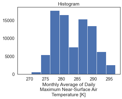

# 绘制切片数据的空间分布
two_months_cali.plot(col='time',col_wrap=1)
plt.show()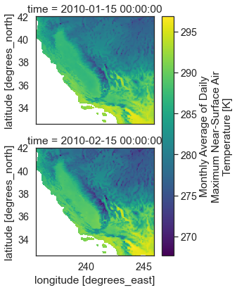

# 若不指定时间范围
cali_ts = monthly_forecast_temp_xr["air_temperature"].sel(lon=slice(aoi_lon[0], aoi_lon[1]),lat=slice(aoi_lat[0], aoi_lat[1]))
cali_ts

提取每个点的每年的最高气温

cali_annual_max=cali_ts.groupby('time.year').max(skipna=True)
cali_annual_max

提取每年的最高气温

cali_annual_max_val=cali_annual_max.groupby('year').max(["lat","lon"])
cali_annual_max_val

绘制每年的最高温变化图

f,ax=plt.subplots(figsize=(12,6))
cali_annual_max_val.plot.line(hue="lat",marker="o",ax=ax,color="grey",markerfacecolor="purple",markeredgecolor="purple")
ax.set(title="Annual Max Temperature (K) in California")
plt.show()

使用Shapefile对nc文件进行切片

在上述的操作中，使用外包络矩形的坐标对nc数据进行了切片，但有时我们希望能得到不规则边界的数据，此时需要使用到regionmask包创建掩膜

f,ax=plt.subplots()
cali_aoi.plot(ax=ax)
ax.set(title="california AOI Subset")plt.show()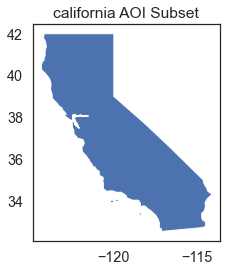

cali_aoi

根据GeoPandasDataFrame生成掩膜

cali_mask=regionmask.mask_3D_geopandas(cali_aoi,monthly_forecast_temp_xr.lon,monthly_forecast_temp_xr.lat)
cali_mask

根据时间和掩膜对数据进行切片

two_months=monthly_forecast_temp_xr.sel(time=slice("2099-10-25","2099-12-15"))two_months=two_months.where(cali_mask)
two_months

绘制掩膜结果

two_months["air_temperature"].plot(col='time',col_wrap=1,figsize=(10, 10))
plt.show()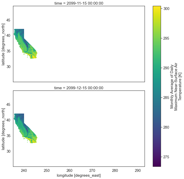

可以看到此时图中显示范围较大，可以通过设置经纬度进一步切片

two_months_masked = monthly_forecast_temp_xr["air_temperature"].sel(time=slice('2099-10-25','2099-12-15'),lon=slice(aoi_lon[0],aoi_lon[1]),lat=slice(aoi_lat[0],aoi_lat[1])).where(cali_mask)
two_months_masked.dims

('time', 'lat', 'lon', 'region')

two_months_masked.plot(col='time', col_wrap=1)
plt.show()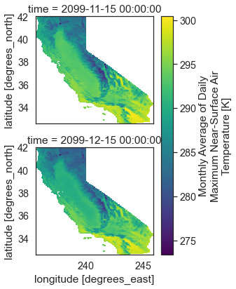

同时对多个区域进行切片

# 选取多个州
cali_or_wash_nev = states_gdf[states_gdf.name.isin(["California", "Oregon", "Washington", "Nevada"])]
cali_or_wash_nev.plot()
plt.show()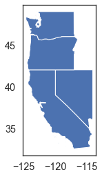

# 根据多个州的范围进行掩膜的生成
west_mask = regionmask.mask_3D_geopandas(cali_or_wash_nev,monthly_forecast_temp_xr.lon,monthly_forecast_temp_xr.lat)
west_mask

帮助生成多个mask的函数

def get_aoi(shp, world=True):"""Takes a geopandas object and converts it to a lat/ lonextent Parameters-----------shp : geopandas objectworld : booleanReturns-------Dictionary of lat and lon spatial bounds"""lon_lat = {}# Get lat min, maxaoi_lat = [float(shp.total_bounds[1]), float(shp.total_bounds[3])]aoi_lon = [float(shp.total_bounds[0]), float(shp.total_bounds[2])]if world:aoi_lon[0] = aoi_lon[0] + 360aoi_lon[1] = aoi_lon[1] + 360lon_lat["lon"] = aoi_lonlon_lat["lat"] = aoi_latreturn lon_latwest_bounds = get_aoi(cali_or_wash_nev)

# 设定提取的起止时间
start_date = "2010-01-15"
end_date = "2010-02-15"# Subset
two_months_west_coast = monthly_forecast_temp_xr["air_temperature"].sel(time=slice(start_date, end_date),lon=slice(west_bounds["lon"][0], west_bounds["lon"][1]),lat=slice(west_bounds["lat"][0], west_bounds["lat"][1]))
two_months_west_coast

two_months_west_coast.plot(col="region",row="time",sharey=False, sharex=False)
plt.show()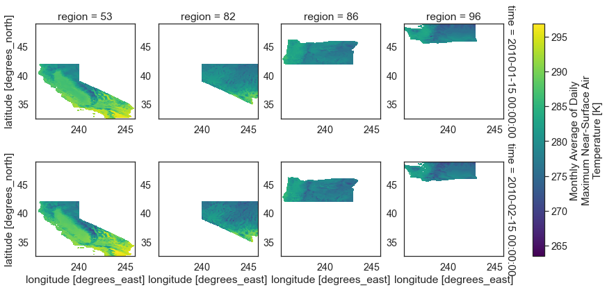

计算每个区域的温度均值

summary = two_months_west_coast.groupby("time").mean(["lat", "lon"])
summary.to_dataframe()

本节完整代码

# 提取geopandas对象的外包络矩形经纬度
def get_aoi(shp, world=True):"""Takes a geopandas object and converts it to a lat/ lonextent """lon_lat = {}# Get lat min, maxaoi_lat = [float(shp.total_bounds[1]), float(shp.total_bounds[3])]aoi_lon = [float(shp.total_bounds[0]), float(shp.total_bounds[2])]# Handle the 0-360 lon valuesif world:aoi_lon[0] = aoi_lon[0] + 360aoi_lon[1] = aoi_lon[1] + 360lon_lat["lon"] = aoi_lonlon_lat["lat"] = aoi_latreturn lon_lat

# 本节完整代码# 读取矢量数据
states_path = "ne_50m_admin_1_states_provinces_lakes"
states_path = os.path.join(states_path, "ne_50m_admin_1_states_provinces_lakes.shp")states_gdf = gpd.read_file(states_path)# 读取nc数据
data_path_monthly = 'http://thredds.northwestknowledge.net:8080/thredds/dodsC/agg_macav2metdata_tasmax_BNU-ESM_r1i1p1_rcp45_2006_2099_CONUS_monthly.nc'
with xr.open_dataset(data_path_monthly) as file_nc:monthly_forecast_temp_xr = file_nc# 数据对象
monthly_forecast_temp_xr# 将geopandas对象转换成掩膜
states_gdf["name"]cali_or_wash_nev = states_gdf[states_gdf.name.isin(["California", "Oregon", "Washington", "Nevada"])]west_mask = regionmask.mask_3D_geopandas(cali_or_wash_nev,monthly_forecast_temp_xr.lon,monthly_forecast_temp_xr.lat)
west_mask
west_bounds = get_aoi(cali_or_wash_nev)# 根据时间、掩膜范围对数据进行切片 .sel().where()
start_date = "2010-01-15"
end_date = "2020-02-15"two_months_west_coast = monthly_forecast_temp_xr["air_temperature"].sel(time=slice(start_date, end_date),lon=slice(west_bounds["lon"][0], west_bounds["lon"][1]),lat=slice(west_bounds["lat"][0], west_bounds["lat"][1])).where(west_mask)# 输出切片数据
two_months_west_coast# 直方图绘制
two_months_west_coast.plot()
plt.show()

# 绘制每个区域的变化
regional_summary = two_months_west_coast.groupby("region").mean(["lat", "lon"])
regional_summary.plot(col="region",marker="o",color="grey",markerfacecolor="purple",markeredgecolor="purple",col_wrap=2)
plt.show()

# 转换为dataframe
two_months_west_coast.groupby("region").mean(["lat", "lon"]).to_dataframe()

参考链接：

https://www.earthdatascience.org/courses/use-data-open-source-python/hierarchical-data-formats-hdf/summarize-climate-data-by-season/

https://gitee.com/jiangroubao/learning/tree/master/NetCDF4

[外链图片转存失败,源站可能有防盗链机制,建议将图片保存下来直接上传(img-yWEE3qlj-1676603621866)(null)]