Mnist分类与气温预测任务
目录
- 传统机器学习与深度学习的特征工程
- 特征向量
- pytorch实现minist代码解析
- 归一化
- 损失函数
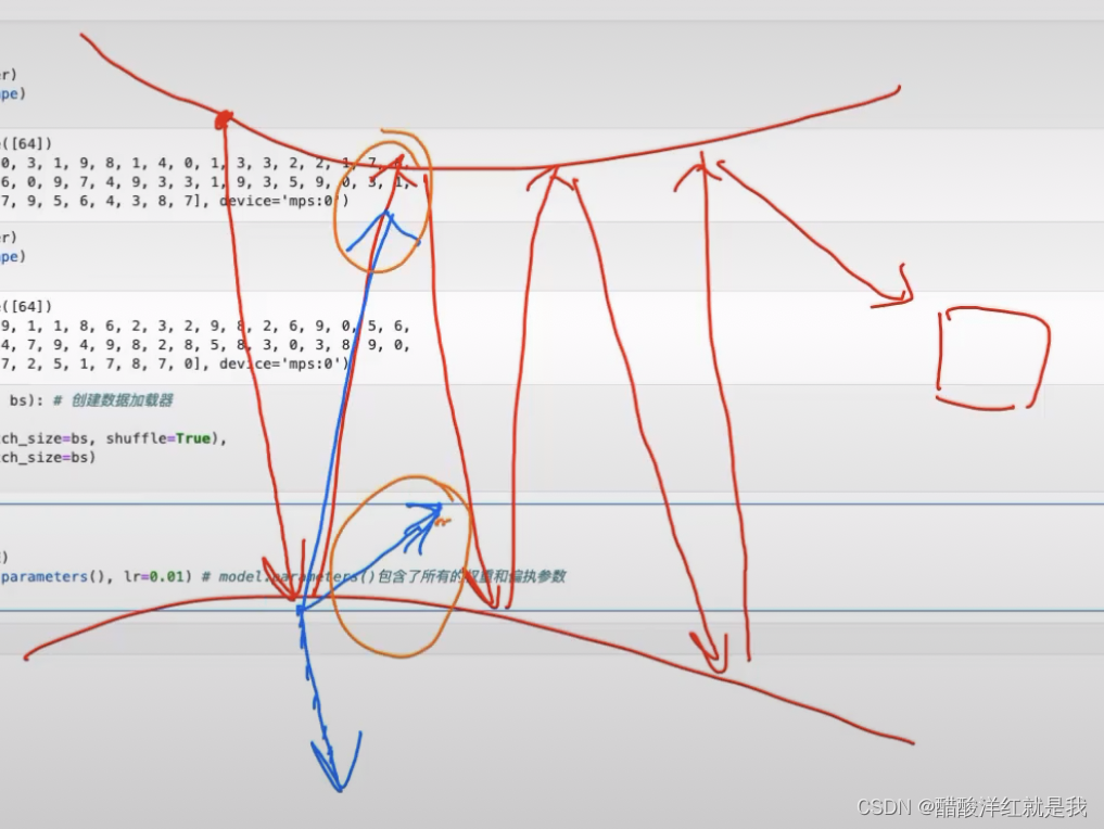
- 计算图
- Mnist分类
- 获取Mnist数据集,预处理,输出一张图像
- 面向工具包编程
- 使用TensorDataset和DataLoader来简化数据预处理
- 计算验证集准确率
- 气温预测
- 回归
- 构建神经网络
- 调包
- 预测训练结果
- 画图对比
传统机器学习与深度学习的特征工程

卷积层:原始输入中间提取有用的一个局部特征
激活函数:用于增加模型的一些非线性,可以让模型学习更加复杂模式
池化层:用于减少数据的维度
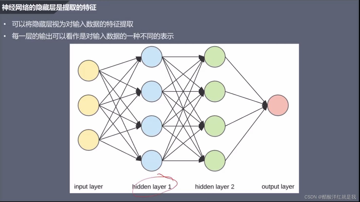
特征向量

pytorch实现minist代码解析
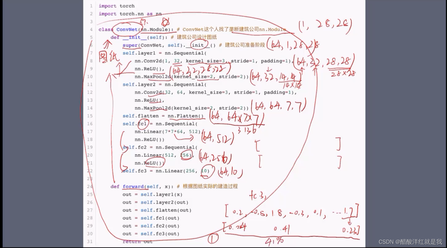
首先继承nn.Module类的一个子类ConvNet,super方法就是在调用nn.Module的一个__init__方法,确保__init__方法中定义的属性和方法都可以在ConvNet中使用
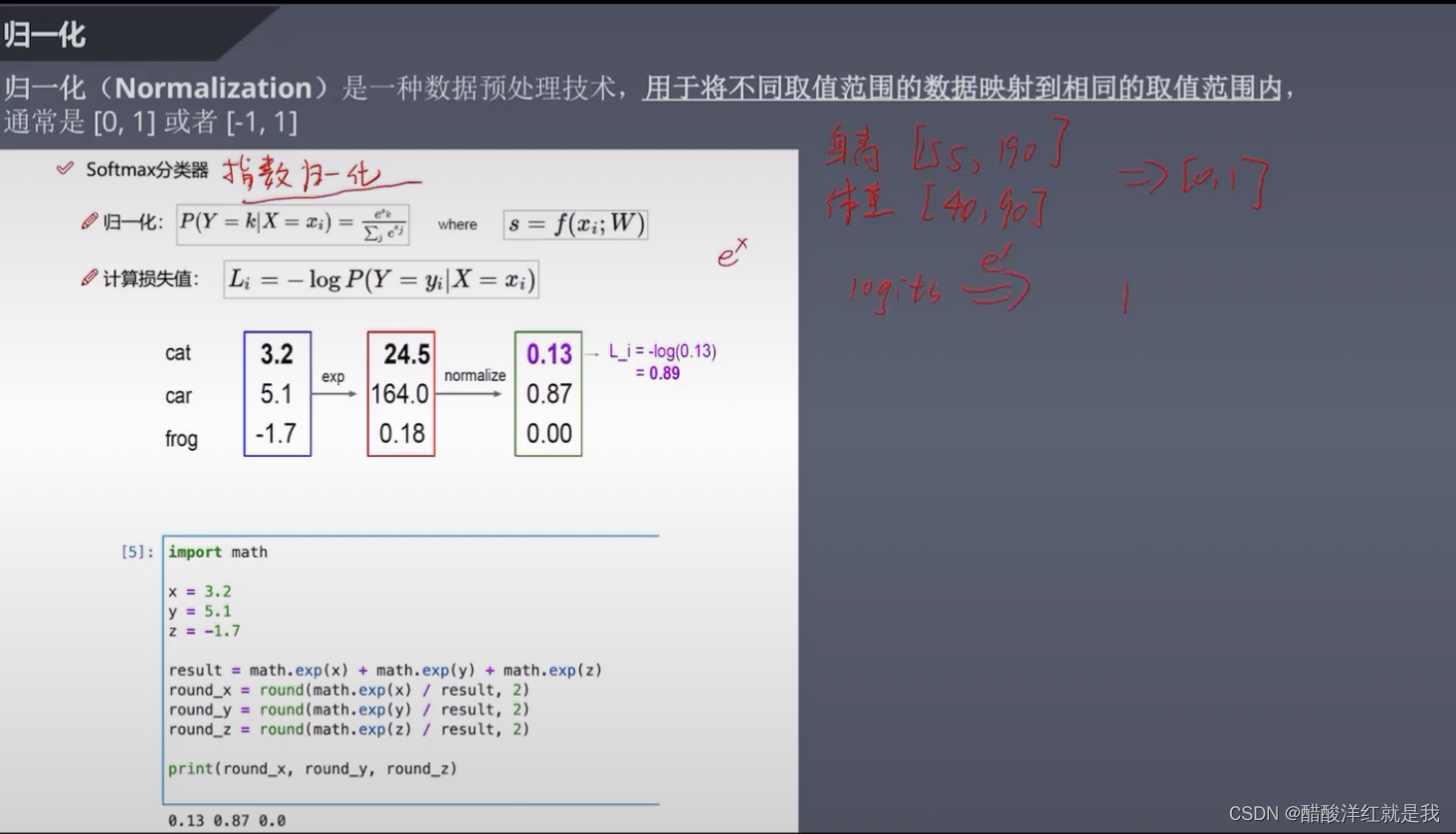
归一化
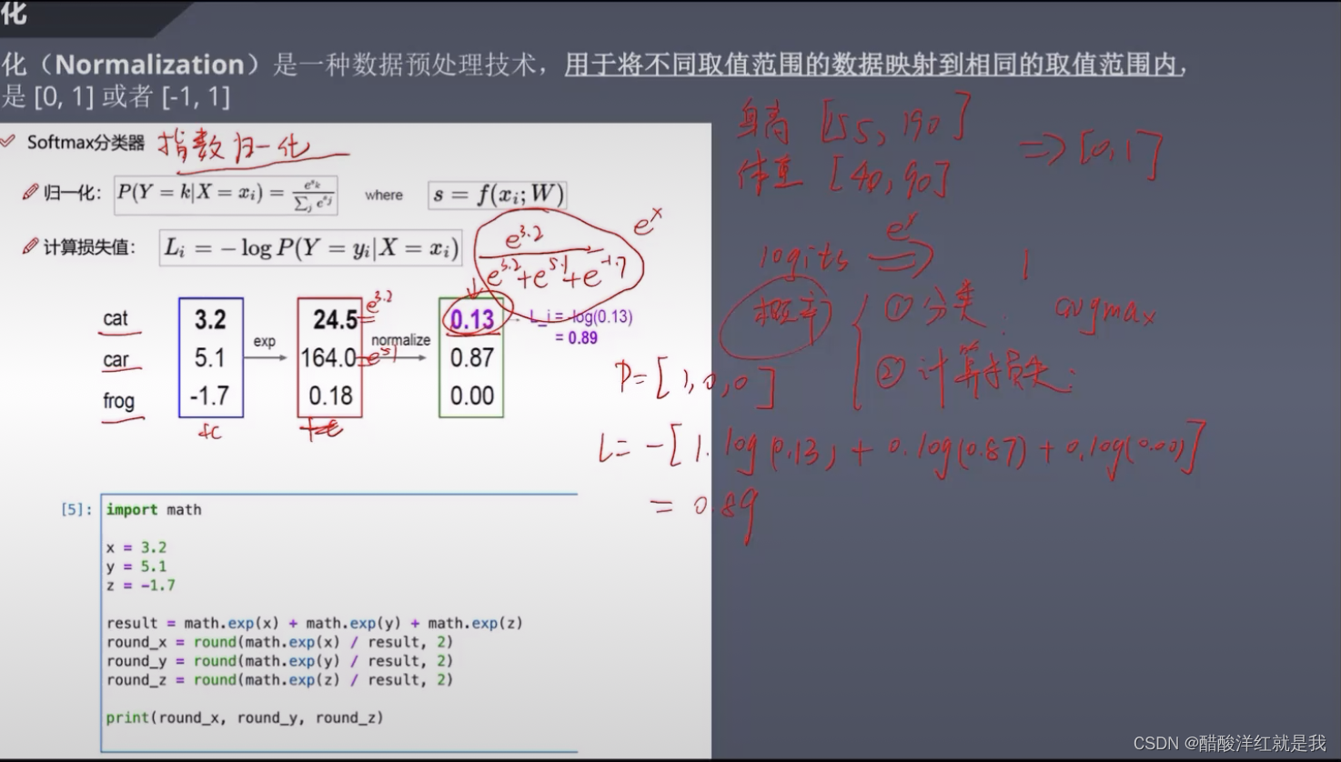
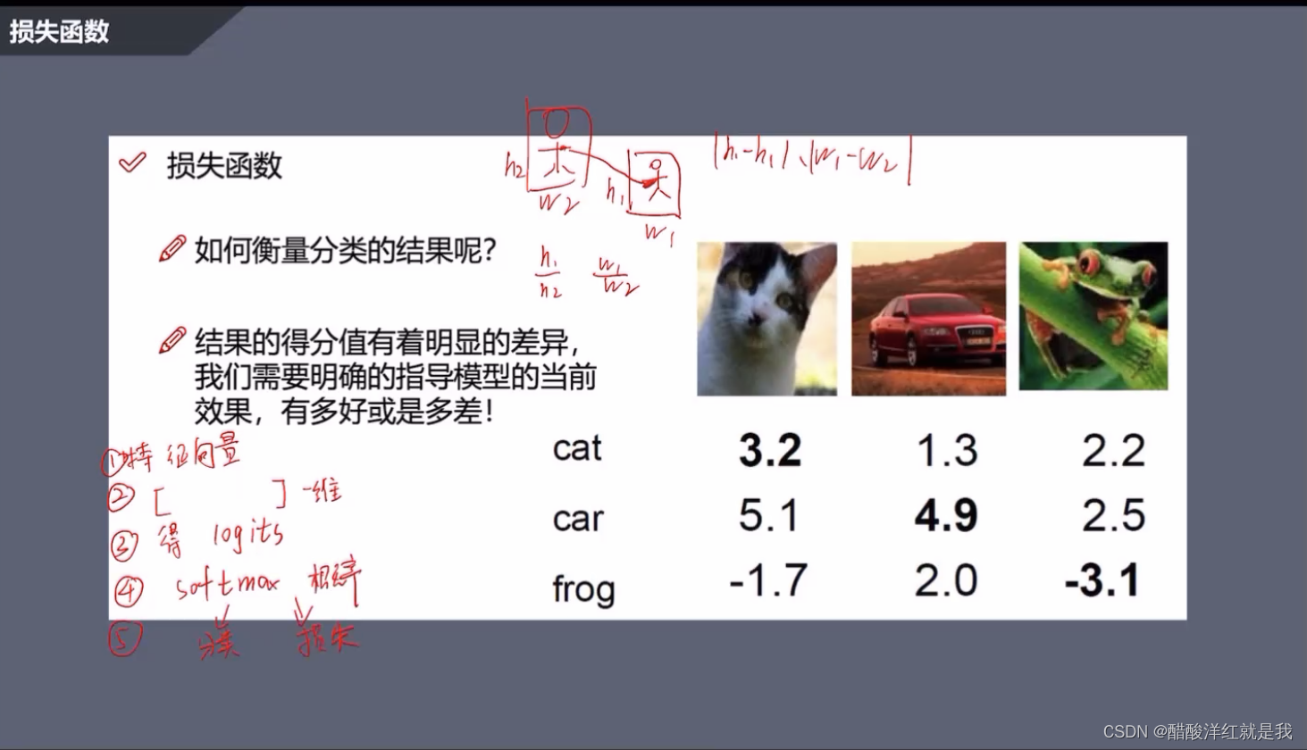
损失函数
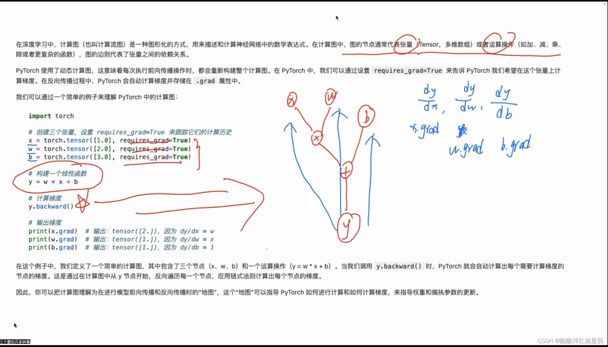
计算图
Mnist分类
获取Mnist数据集,预处理,输出一张图像
import torch
print(torch.__version__)
#win用户
DEVICE=torch.device('cuda' if torch.cuda.is_available() else 'cpu')
#mac用户
DEVICE=torch.device('mps' if torch.backends.mps.is_available() else 'cpu')
print('当前设备',DEVICE)

#将图像嵌入输出的单元格
%matplotlib inline
from pathlib import Path # 处理文件路径
import requestsDATA_PATH = Path("data")
PATH = DATA_PATH / "mnist"
PATH.mkdir(parents=True, exist_ok=True)URL = "http://deeplearning.net/data/mnist/"
FILENAME = "mnist.pkl.gz"if not (PATH / FILENAME).exists():content = requests.get(URL + FILENAME).content(PATH / FILENAME).open("wb").write(content)
import pickle
import gzipwith gzip.open((PATH / FILENAME).as_posix(), "rb") as f:((x_train, y_train), (x_valid, y_valid), (x_test, y_test)) = pickle.load(f, encoding="latin-1")
print("x_train: ", type(x_train), x_train.dtype, x_train.size, x_train.shape, "; y_train: ", y_train.shape)

print("x_valid: ", type(x_valid), x_valid.dtype, x_valid.size, x_valid.shape, "; y_valid: ", y_valid.shape)

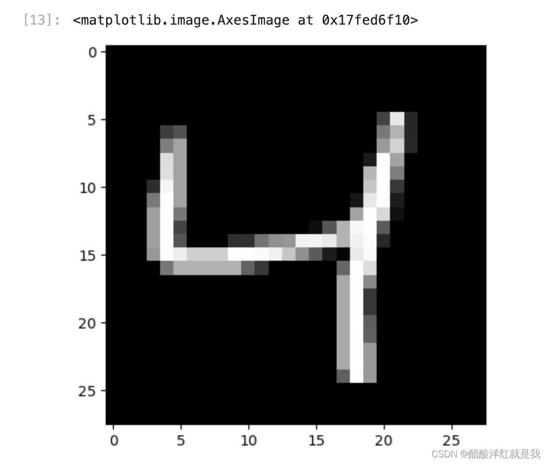
from matplotlib import pyplotpyplot.imshow(x_train[2].reshape((28, 28)), cmap="gray")
y_train[:10]

x_train, y_train, x_valid, y_valid = map(lambda x: torch.tensor(x, device=DEVICE),(x_train, y_train, x_valid, y_valid)
)
print("x_train: ", x_train, "; y_train: ", y_train)
x_train[0]
import torch.nn.functional as Floss_func = F.cross_entropy # 损失函数,传入预测、真实值的标签def model(xb):xb = xb.to(DEVICE)return xb.mm(weights) + bias # x*w+b
bs = 64xb = x_train[0:bs] # 64, 784yb = y_train[0:bs] # 真实标签weights = torch.randn([784, 10], dtype = torch.float, requires_grad = True)bias = torch.zeros(10, requires_grad = True)weights = weights.to(DEVICE)
bias = bias.to(DEVICE)print(loss_func(model(xb), yb))

补充:关于map函数的例子
def square(x):return x**2
numbers=[1,2,3,4,5]
squares=map(square,numbers)
print(list(squares))

也就是map函数第一个参数是函数,第二个参数是数值,将函数作用于数值
面向工具包编程
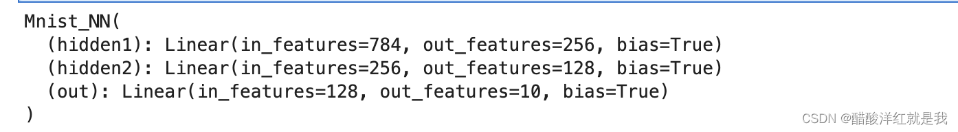
from torch import nn # 提供神经网网络的类和函数 ,nn.Moduleclass Mnist_NN(nn.Module):def __init__(self): # 设计房屋图纸super(Mnist_NN, self).__init__()self.hidden1 = nn.Linear(784, 256) # 784-输入层,256-隐藏层1self.hidden2 = nn.Linear(256, 128)self.out = nn.Linear(128, 10)def forward(self, x): # 实际造房子x2 = F.relu(self.hidden1(x)) # x: [bs, 784], w1: [784, 256], b1: [256] -> x2:[bs,256]x3 = F.relu(self.hidden2(x2)) # x2: [bs, 256], w2:[256, 128], b2[128] -> x3[bs, 128]x_out = self.out(x3) # x3: [bs, 128], w3: [128, 10], b3[10] -> x_out: [bs, 10]return x_out
net = Mnist_NN().to(DEVICE)
print(net)
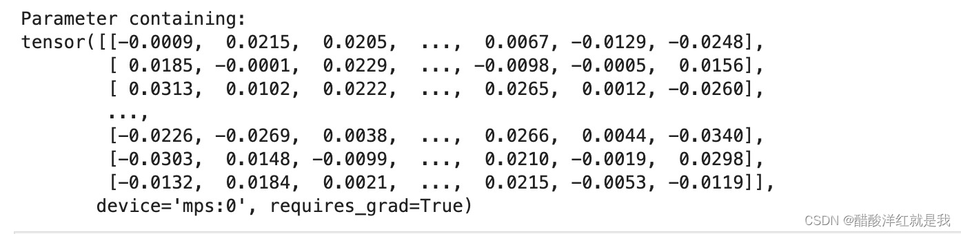
print(net.hidden1.weight)
for name, parameter in net.named_parameters():print(name, parameter)
使用TensorDataset和DataLoader来简化数据预处理
from torch.utils.data import TensorDatasetfrom torch.utils.data import DataLoadertrain_ds = TensorDataset(x_train, y_train) #torch.utils.data.Dataset
train_dl = DataLoader(train_ds, batch_size=64, shuffle=True)valid_ds = TensorDataset(x_valid, y_valid)
valid_dl = DataLoader(valid_ds, batch_size=bs)
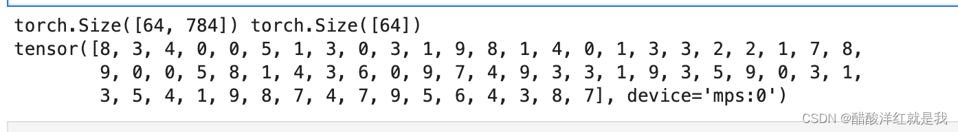
data_iter = iter(train_dl)batch_x, batch_y = next(data_iter)
print(batch_x.shape, batch_y.shape)
print(batch_y)
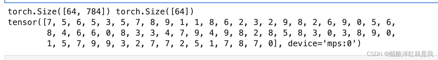
batch_x, batch_y = next(data_iter)
print(batch_x.shape, batch_y.shape)
print(batch_y)
def get_data(train_bs, valid_bs, bs): # 创建数据加载器return (DataLoader(train_ds, batch_size=bs, shuffle=True),DataLoader(valid_ds, batch_size=bs))
from torch import optim
def get_model():model = Mnist_NN().to(DEVICE)optimizer = optim.SGD(model.parameters(), lr=0.01) # model.parameters()包含了所有的权重和偏执参数return model, optimizer
注:adam相比于SGD是引入了一个惯性,相当于一个平行四边形的一个合成法则
def loss_batch(model, loss_func, xb, yb, opt=None):loss = loss_func(model(xb), yb)if opt is not None: # 此时是训练集opt.zero_grad()loss.backward()opt.step()return loss.item(), len(xb)
opt为True是训练集测试损失,opt为None是验证集测试损失
def loss_batch(model, loss_func, xb, yb, opt=None):loss = loss_func(model(xb), yb)if opt is not None: # 此时是训练集opt.zero_grad()loss.backward()opt.step()return loss.item(), len(xb)
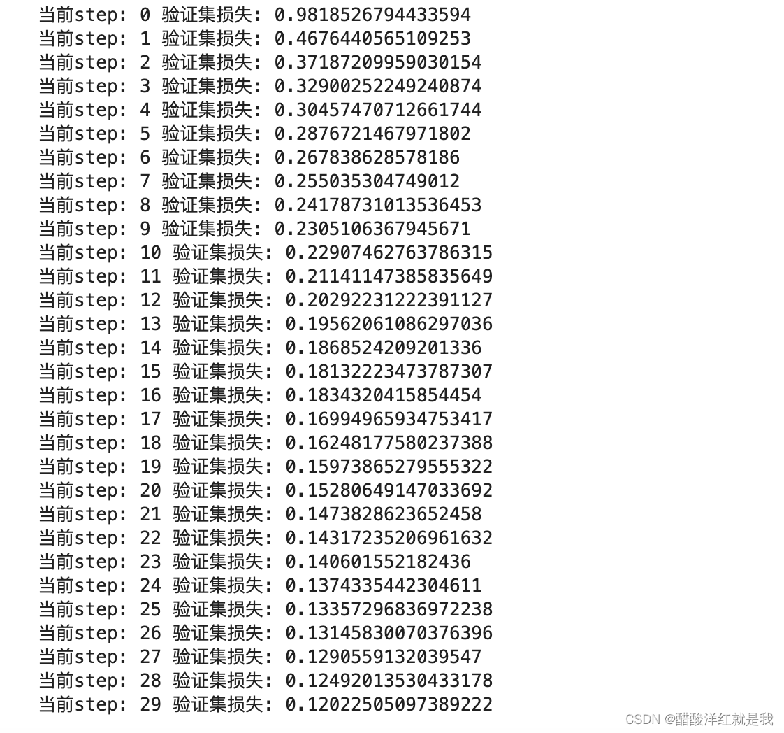
import numpy as npdef fit(epoch, model, loss_func, opt, train_dl, valid_dl):for step in range(epoch):model.train()for xb, yb in train_dl:loss_batch(model, loss_func, xb, yb, opt)model.eval() # 考试with torch.no_grad():losses, nums = zip(*[loss_batch(model, loss_func, xb, yb) for xb, yb in valid_dl] # "*"——解包/解开)# print(f"losses: {losses}")# print(f"nums: {nums}")val_loss = np.sum(np.multiply(losses, nums)) / np.sum(nums) # 加权平均损失print('当前step: '+str(step), '验证集损失: '+str(val_loss))
train_dl, valid_dl = get_data(train_ds, valid_ds, bs=64)
model, optimizer = get_model()
fit(30, model, loss_func, optimizer, train_dl, valid_dl)
计算验证集准确率
torch.set_printoptions(precision=4, sci_mode=False)
for xb, yb in valid_dl:output = model(xb)print(output)print(output.shape)break
for xb, yb in valid_dl:output = model(xb)probs = torch.softmax(output, dim=1)print(probs)print(probs.shape)break
for xb, yb in valid_dl:output = model(xb)probs = torch.softmax(output, dim=1)preds = torch.argmax(probs, dim=1)print(preds)print(preds.shape)break
correct_predict = 0 # 计数正确预测图片的数目
total_quantity = 0 # 计数验证集总数for xb, yb in valid_dl:output = model(xb)probs = torch.softmax(output, dim=1)preds = torch.argmax(probs, dim=1)total_quantity += yb.size(0)# print(yb.size(0))# print((preds == yb).sum())# print((preds == yb).sum().item())correct_predict += (preds == yb).sum().item()print(f"验证集的准确率是: {100 * correct_predict / total_quantity} % ")

气温预测
回归
import numpy as np # 矩阵运算
import pandas as pd
import matplotlib.pyplot as plt
import torch
import torch.optim as optimimport warnings
warnings.filterwarnings("ignore")%matplotlib inline
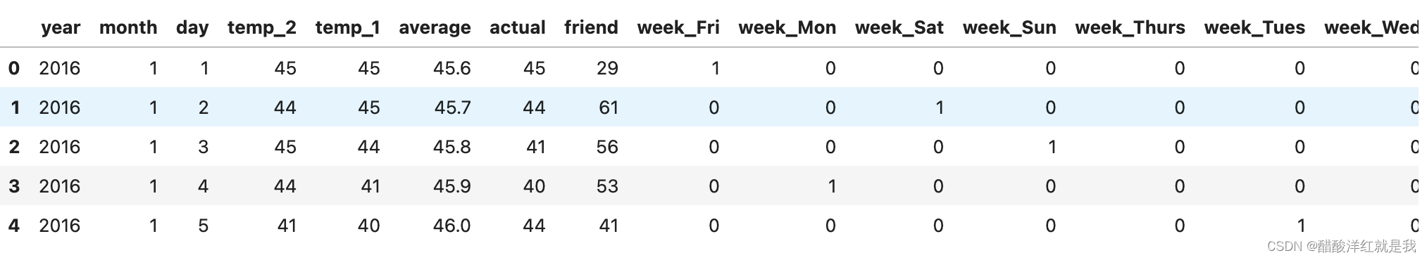
features = pd.read_csv('temps.csv')features.head()
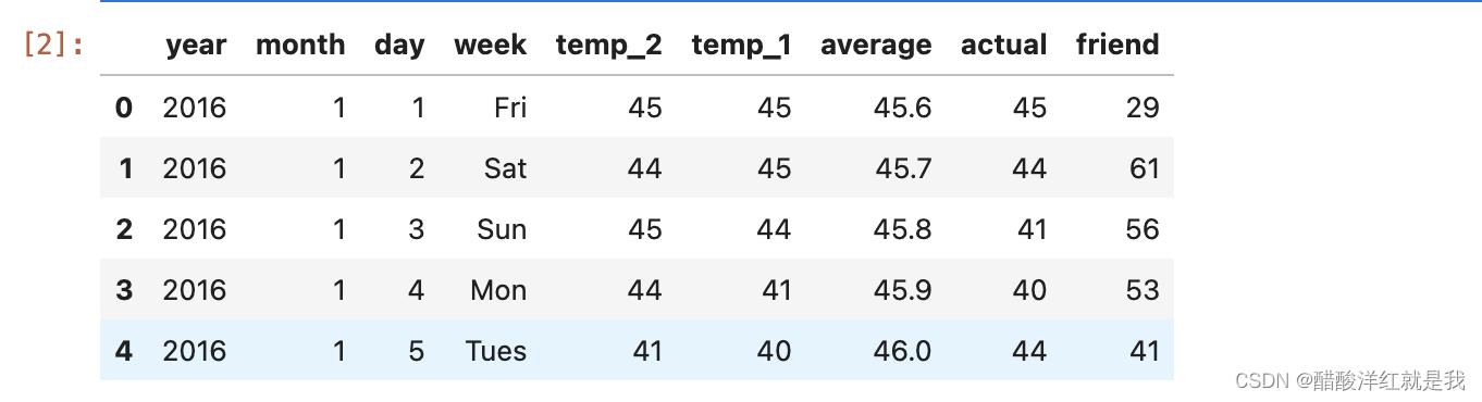
print("数据维度: ", features.shape)

# 处理时间数据
import datetimeyears = features['year']
months = features['month']
days = features['day']dates = [str(int(year)) + '-' + str(int(month)) + '-' + str(int(day)) for year, month, day in zip(years, months, days)]
dates[:5]

dates = [str(int(year)) + '-' + str(int(month)) + '-' + str(int(day)) for year, month, day in zip(years, months, days)]
dates = [datetime.datetime.strptime(date, '%Y-%m-%d') for date in dates]
dates[:5]

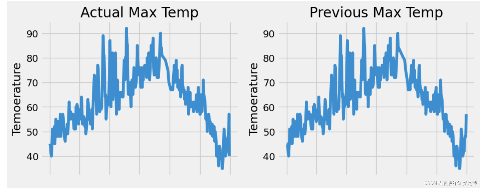
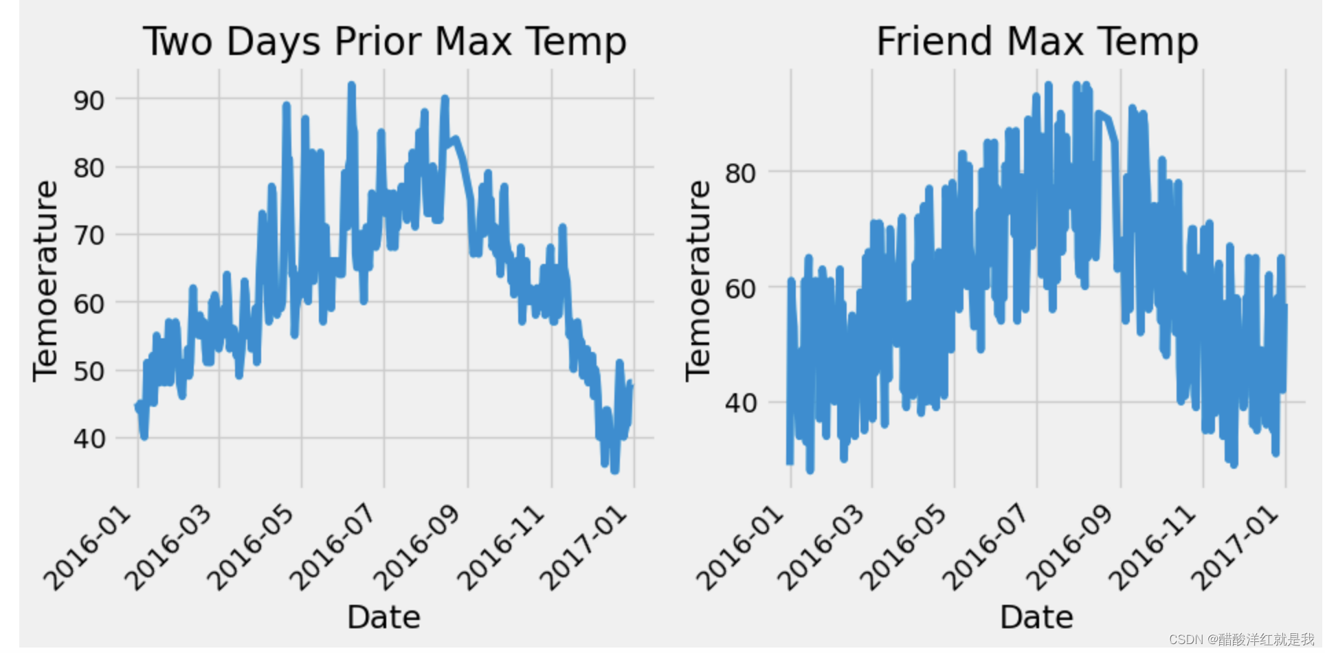
plt.style.use('fivethirtyeight')fig, ((ax1, ax2), (ax3, ax4)) = plt.subplots(nrows=2, ncols=2, figsize = (10, 10))
fig.autofmt_xdate(rotation=45) #x轴翻转45度# 标签值
ax1.plot(dates, features['actual'])
ax1.set_xlabel(''); ax1.set_ylabel('Temoerature'); ax1.set_title('Actual Max Temp')# 昨天温度
ax2.plot(dates, features['temp_1'])
ax2.set_xlabel(''); ax2.set_ylabel('Temoerature'); ax2.set_title('Previous Max Temp')# 前天温度
ax3.plot(dates, features['temp_2'])
ax3.set_xlabel('Date'); ax3.set_ylabel('Temoerature'); ax3.set_title('Two Days Prior Max Temp')# 朋友预测温度
ax4.plot(dates, features['friend'])
ax4.set_xlabel('Date'); ax4.set_ylabel('Temoerature'); ax4.set_title('Friend Max Temp')
features = pd.get_dummies(features)
features.head()
labels = np.array(features['actual'])# 在特征中去掉标签
features = features.drop('actual', axis=1)feature_list = list(features.columns)features = np.array(features)
features.shape

from sklearn import preprocessing
input_features = preprocessing.StandardScaler().fit_transform(features)
input_features[:5]
构建神经网络
x = torch.tensor(input_features, dtype = float)
y = torch.tensor(labels, dtype=float)
print(x.shape, y.shape)
# 权重初始化
weights = torch.randn((14, 128), dtype = float, requires_grad = True)
biases = torch.randn(128, dtype = float, requires_grad = True)
weights2 = torch.randn((128, 1), dtype = float, requires_grad = True)
biases2 = torch.randn(1, dtype = float, requires_grad = True) learning_rate = 0.001
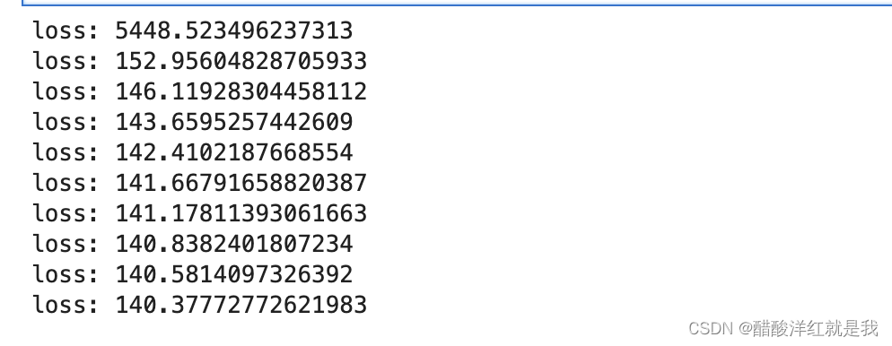
losses = []for i in range(1000):hidden = x.mm(weights) + biaseshidden = torch.relu(hidden)predictions = hidden.mm(weights2) + biases2loss = torch.mean((predictions - y)**2)losses.append(loss.item())if i % 100 == 0:print(f"loss: {loss}")# 反向传播loss.backward()# 更新,相当于optim.step()weights.data.add_(- learning_rate * weights.grad.data) biases.data.add_(- learning_rate * biases.grad.data)weights2.data.add_(- learning_rate * weights2.grad.data)biases2.data.add_(- learning_rate * biases2.grad.data)# 清空梯度,optim.zero_grad()weights.grad.data.zero_()biases.grad.data.zero_()weights2.grad.data.zero_()biases2.grad.data.zero_()
调包
import torch.optim as optim# 数据准备
# 将数据都转化为tensor张量
x = torch.tensor(input_features, dtype = torch.float)
y = torch.tensor(labels, dtype=torch.float).view(-1, 1) # 改成(n, 1)
print(x.shape, y.shape)
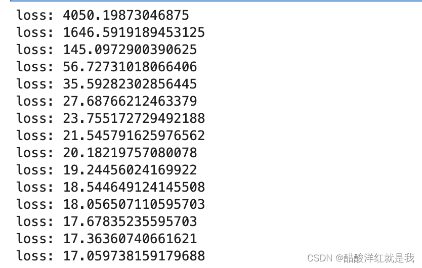
model = torch.nn.Sequential(torch.nn.Linear(14, 128),torch.nn.ReLU(),torch.nn.Linear(128, 1)
)# 均方误差MSE
criterion = torch.nn.MSELoss(reduction='mean')optimizer = optim.Adam(model.parameters(), lr=0.001)losses = [] # 存储每一次迭代的损失for i in range(3000):predictions = model(x) # [348, 1]loss = criterion(predictions, y)losses.append(loss.item())if i % 200 == 0:print(f"loss: {loss.item()}")optimizer.zero_grad()loss.backward()optimizer.step()
预测训练结果
x = torch.tensor(input_features, dtype = torch.float)
predict = model(x).data.numpy()
dates = [str(int(year)) + '-' + str(int(month)) + '-' + str(int(day)) for year, month, day in zip(years, months, days)]
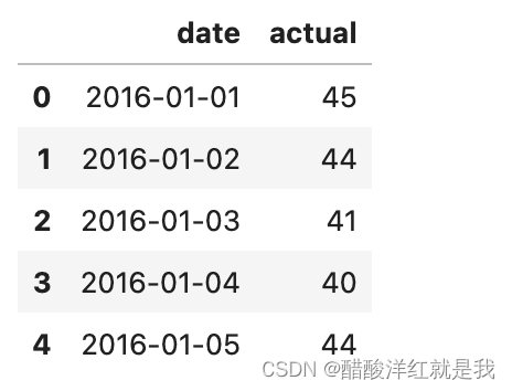
dates = [datetime.datetime.strptime(date, '%Y-%m-%d') for date in dates]# 创建一个表格来存日期和对应的真实标签
true_data = pd.DataFrame(data = {'date': dates, 'actual': labels})# 创建一个表格来存日期和对应的预测值
predictions_data = pd.DataFrame(data = {'date': dates, 'prediction': predict.reshape(-1)})predict.shape, predict.reshape(-1).shape

true_data[:5]
predictions_data[:5]

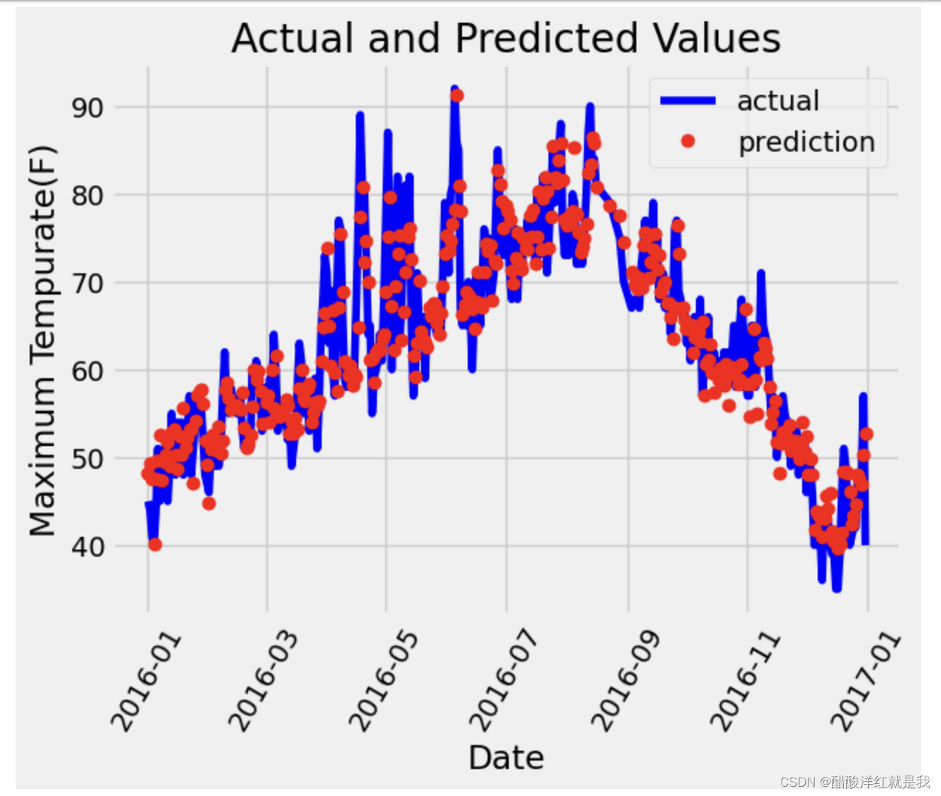
画图对比
# 真实值
plt.plot(true_data['date'], true_data['actual'], 'b-', label = "actual")# 预测值
plt.plot(predictions_data['date'], predictions_data['prediction'], 'ro', label = "prediction")plt.xticks(rotation = 60)plt.legend()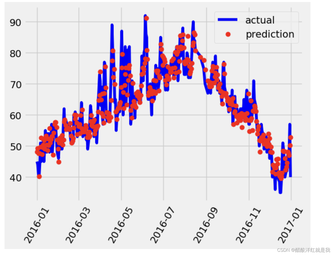
# 真实值
plt.plot(true_data['date'], true_data['actual'], 'b-', label = "actual")# 预测值
plt.plot(predictions_data['date'], predictions_data['prediction'], 'ro', label = "prediction")plt.xticks(rotation = 60)plt.legend()plt.xlabel('Date'); plt.ylabel('Maximum Tempurate(F)'); plt.title('Actual and Predicted Values')