【Python机器学习】实验04(2) 机器学习应用实践--手动调参
文章目录
- 机器学习应用实践
- 1.1 准备数据
- 此处进行的调整为:要所有数据进行拆分
- 1.2 定义假设函数
- Sigmoid 函数
- 1.3 定义代价函数
- 1.4 定义梯度下降算法
- gradient descent(梯度下降)
- 此处进行的调整为:采用train_x, train_y进行训练
- 1.5 绘制决策边界
- 1.6 计算准确率
- 此处进行的调整为:采用X_test和y_test来测试进行训练
- 1.7 试试用Sklearn来解决
- 此处进行的调整为:采用X_train和y_train进行训练
- 此处进行的调整为:采用X_test和y_test进行训练
- 1.8 如何选择超参数?比如多少轮迭代次数好?
- 1.9 如何选择超参数?比如学习率设置多少好?
- 1.10 如何选择超参数?试试调整l2正则化因子
- 实验4(2) 完成正则化因子的调参,下面给出了正则化因子lambda的范围,请参照学习率的调参,完成下面代码
机器学习应用实践
上一次练习中,我们采用逻辑回归并且应用到一个分类任务。
但是,我们用训练数据训练了模型,然后又用训练数据来测试模型,是否客观?接下来,我们仅对实验1的数据划分进行修改
需要改的地方为:下面红色部分给出了具体的修改。
1 训练数据数量将会变少
2 评估模型时要采用测试集
1.1 准备数据
本实验的数据包含两个变量(评分1和评分2,可以看作是特征),某大学的管理者,想通过申请学生两次测试的评分,来决定他们是否被录取。因此,构建一个可以基于两次测试评分来评估录取可能性的分类模型。
import numpy as np
import pandas as pd
import matplotlib.pyplot as plt
#利用pandas显示数据
path = 'ex2data1.txt'
data = pd.read_csv(path, header=None, names=['Exam1', 'Exam2', 'Admitted'])
data.head()
| Exam1 | Exam2 | Admitted | |
|---|---|---|---|
| 0 | 34.623660 | 78.024693 | 0 |
| 1 | 30.286711 | 43.894998 | 0 |
| 2 | 35.847409 | 72.902198 | 0 |
| 3 | 60.182599 | 86.308552 | 1 |
| 4 | 79.032736 | 75.344376 | 1 |
positive=data[data["Admitted"].isin([1])]
negative=data[data["Admitted"].isin([0])]
#准备训练数据
col_num=data.shape[1]
X=data.iloc[:,:col_num-1]
y=data.iloc[:,col_num-1]
X.insert(0,"ones",1)
X.shape
(100, 3)
X=X.values
X.shape
(100, 3)
y=y.values
y.shape
(100,)
此处进行的调整为:要所有数据进行拆分
from sklearn.model_selection import train_test_split
X_train, X_test, y_train, y_test =train_test_split(X,y,test_size=0.2,random_state=0)
train_x,test_x,train_y,test_y
(array([[ 1. , 82.36875376, 40.61825516],[ 1. , 56.2538175 , 39.26147251],[ 1. , 60.18259939, 86.3085521 ],[ 1. , 64.03932042, 78.03168802],[ 1. , 62.22267576, 52.06099195],[ 1. , 62.0730638 , 96.76882412],[ 1. , 61.10666454, 96.51142588],[ 1. , 74.775893 , 89.5298129 ],[ 1. , 67.31925747, 66.58935318],[ 1. , 47.26426911, 88.475865 ],[ 1. , 75.39561147, 85.75993667],[ 1. , 88.91389642, 69.8037889 ],[ 1. , 94.09433113, 77.15910509],[ 1. , 80.27957401, 92.11606081],[ 1. , 99.27252693, 60.999031 ],[ 1. , 93.1143888 , 38.80067034],[ 1. , 70.66150955, 92.92713789],[ 1. , 97.64563396, 68.86157272],[ 1. , 30.05882245, 49.59297387],[ 1. , 58.84095622, 75.85844831],[ 1. , 30.28671077, 43.89499752],[ 1. , 35.28611282, 47.02051395],[ 1. , 94.44336777, 65.56892161],[ 1. , 51.54772027, 46.85629026],[ 1. , 79.03273605, 75.34437644],[ 1. , 53.97105215, 89.20735014],[ 1. , 67.94685548, 46.67857411],[ 1. , 83.90239366, 56.30804622],[ 1. , 74.78925296, 41.57341523],[ 1. , 45.08327748, 56.31637178],[ 1. , 90.44855097, 87.50879176],[ 1. , 71.79646206, 78.45356225],[ 1. , 34.62365962, 78.02469282],[ 1. , 40.23689374, 71.16774802],[ 1. , 61.83020602, 50.25610789],[ 1. , 79.94481794, 74.16311935],[ 1. , 75.01365839, 30.60326323],[ 1. , 54.63510555, 52.21388588],[ 1. , 34.21206098, 44.2095286 ],[ 1. , 90.54671411, 43.39060181],[ 1. , 95.86155507, 38.22527806],[ 1. , 85.40451939, 57.05198398],[ 1. , 40.45755098, 97.53518549],[ 1. , 32.57720017, 95.59854761],[ 1. , 82.22666158, 42.71987854],[ 1. , 68.46852179, 85.5943071 ],[ 1. , 52.10797973, 63.12762377],[ 1. , 80.366756 , 90.9601479 ],[ 1. , 39.53833914, 76.03681085],[ 1. , 52.34800399, 60.76950526],[ 1. , 76.97878373, 47.57596365],[ 1. , 38.7858038 , 64.99568096],[ 1. , 91.5649745 , 88.69629255],[ 1. , 99.31500881, 68.77540947],[ 1. , 55.34001756, 64.93193801],[ 1. , 66.74671857, 60.99139403],[ 1. , 67.37202755, 42.83843832],[ 1. , 89.84580671, 45.35828361],[ 1. , 72.34649423, 96.22759297],[ 1. , 50.4581598 , 75.80985953],[ 1. , 62.27101367, 69.95445795],[ 1. , 64.17698887, 80.90806059],[ 1. , 94.83450672, 45.6943068 ],[ 1. , 77.19303493, 70.4582 ],[ 1. , 34.18364003, 75.23772034],[ 1. , 66.56089447, 41.09209808],[ 1. , 74.24869137, 69.82457123],[ 1. , 82.30705337, 76.4819633 ],[ 1. , 78.63542435, 96.64742717],[ 1. , 32.72283304, 43.30717306],[ 1. , 75.47770201, 90.424539 ],[ 1. , 33.91550011, 98.86943574],[ 1. , 89.67677575, 65.79936593],[ 1. , 57.23870632, 59.51428198],[ 1. , 84.43281996, 43.53339331],[ 1. , 42.26170081, 87.10385094],[ 1. , 49.07256322, 51.88321182],[ 1. , 44.66826172, 66.45008615],[ 1. , 97.77159928, 86.72782233],[ 1. , 51.04775177, 45.82270146]]),array([0, 0, 1, 1, 0, 1, 1, 1, 1, 1, 1, 1, 1, 1, 1, 0, 1, 1, 0, 1, 0, 0,1, 0, 1, 1, 0, 1, 0, 0, 1, 1, 0, 0, 0, 1, 0, 0, 0, 1, 0, 1, 1, 0,0, 1, 0, 1, 0, 0, 1, 0, 1, 1, 1, 1, 0, 1, 1, 1, 1, 1, 1, 1, 0, 0,1, 1, 1, 0, 1, 0, 1, 1, 1, 1, 0, 0, 1, 0], dtype=int64),array([[ 1. , 80.19018075, 44.82162893],[ 1. , 42.07545454, 78.844786 ],[ 1. , 35.84740877, 72.90219803],[ 1. , 49.58667722, 59.80895099],[ 1. , 99.8278578 , 72.36925193],[ 1. , 74.49269242, 84.84513685],[ 1. , 69.07014406, 52.74046973],[ 1. , 60.45788574, 73.0949981 ],[ 1. , 50.28649612, 49.80453881],[ 1. , 83.48916274, 48.3802858 ],[ 1. , 34.52451385, 60.39634246],[ 1. , 55.48216114, 35.57070347],[ 1. , 60.45555629, 42.50840944],[ 1. , 69.36458876, 97.71869196],[ 1. , 75.02474557, 46.55401354],[ 1. , 61.37928945, 72.80788731],[ 1. , 50.53478829, 48.85581153],[ 1. , 77.92409145, 68.97235999],[ 1. , 52.04540477, 69.43286012],[ 1. , 76.0987867 , 87.42056972]]),array([1, 0, 0, 0, 1, 1, 1, 1, 0, 1, 0, 0, 0, 1, 1, 1, 0, 1, 1, 1],dtype=int64))
X_train.shape, X_test.shape, y_train.shape, y_test.shape
((80, 3), (20, 3), (80,), (20,))
train_x.shape,train_y.shape
((80, 3), (20, 3))
1.2 定义假设函数
Sigmoid 函数
g g g 代表一个常用的逻辑函数(logistic function)为 S S S形函数(Sigmoid function),公式为: g ( z ) = 1 1 + e − z g\left( z \right)=\frac{1}{1+{{e}^{-z}}} g(z)=1+e−z1
合起来,我们得到逻辑回归模型的假设函数:
h ( x ) = 1 1 + e − w T x {{h}}\left( x \right)=\frac{1}{1+{{e}^{-{{w }^{T}}x}}} h(x)=1+e−wTx1
def sigmoid(z):return 1 / (1 + np.exp(-z))
让我们做一个快速的检查,来确保它可以工作。
w=np.zeros((X.shape[1],1))
#定义假设函数h(x)=1/(1+exp^(-w.Tx))
def h(X,w):z=X@wh=sigmoid(z)return h
1.3 定义代价函数
y_hat=sigmoid(X@w)
X.shape,y.shape,np.log(y_hat).shape
((100, 3), (100,), (100, 1))
现在,我们需要编写代价函数来评估结果。
代价函数:
J ( w ) = − 1 m ∑ i = 1 m ( y ( i ) log ( h ( x ( i ) ) ) + ( 1 − y ( i ) ) log ( 1 − h ( x ( i ) ) ) ) J\left(w\right)=-\frac{1}{m}\sum\limits_{i=1}^{m}{({{y}^{(i)}}\log \left( {h}\left( {{x}^{(i)}} \right) \right)+\left( 1-{{y}^{(i)}} \right)\log \left( 1-{h}\left( {{x}^{(i)}} \right) \right))} J(w)=−m1i=1∑m(y(i)log(h(x(i)))+(1−y(i))log(1−h(x(i))))
#代价函数构造
def cost(X,w,y):#当X(m,n+1),y(m,),w(n+1,1)y_hat=h(X,w)right=np.multiply(y.ravel(),np.log(y_hat).ravel())+np.multiply((1-y).ravel(),np.log(1-y_hat).ravel())cost=-np.sum(right)/X.shape[0]return cost
#设置初始的权值
w=np.zeros((X.shape[1],1))
#查看初始的代价
cost(X,w,y)
0.6931471805599453
看起来不错,接下来,我们需要一个函数来计算我们的训练数据、标签和一些参数 w w w的梯度。
1.4 定义梯度下降算法
gradient descent(梯度下降)
- 这是批量梯度下降(batch gradient descent)
- 转化为向量化计算: 1 m X T ( S i g m o i d ( X W ) − y ) \frac{1}{m} X^T( Sigmoid(XW) - y ) m1XT(Sigmoid(XW)−y)
∂ J ( w ) ∂ w j = 1 m ∑ i = 1 m ( h ( x ( i ) ) − y ( i ) ) x j ( i ) \frac{\partial J\left( w \right)}{\partial {{w }_{j}}}=\frac{1}{m}\sum\limits_{i=1}^{m}{({{h}}\left( {{x}^{(i)}} \right)-{{y}^{(i)}})x_{_{j}}^{(i)}} ∂wj∂J(w)=m1i=1∑m(h(x(i))−y(i))xj(i)
h(X,w).shape
(100, 1)
def grandient(X,y,iter_num,alpha):y=y.reshape((X.shape[0],1))w=np.zeros((X.shape[1],1))cost_lst=[]for i in range(iter_num):y_pred=h(X,w)-ytemp=np.zeros((X.shape[1],1))for j in range(X.shape[1]):right=np.multiply(y_pred.ravel(),X[:,j])gradient=1/(X.shape[0])*(np.sum(right))temp[j,0]=w[j,0]-alpha*gradientw=tempcost_lst.append(cost(X,w,y.ravel()))return w,cost_lst
此处进行的调整为:采用train_x, train_y进行训练
train_x.shape,train_y.shape
((80, 3), (20, 3))
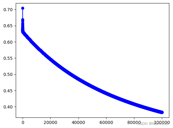
iter_num,alpha=100000,0.001
w,cost_lst=grandient(X_train, y_train,iter_num,alpha)
cost_lst[iter_num-1]
0.38273008292061245
plt.plot(range(iter_num),cost_lst,"b-o")
[<matplotlib.lines.Line2D at 0x1d0f1417d30>]
Xw—X(m,n) w (n,1)
w
array([[-4.86722837],[ 0.04073083],[ 0.04257751]])
1.5 绘制决策边界
高维数据的决策边界无法可视化
1.6 计算准确率
此处进行的调整为:采用X_test和y_test来测试进行训练
如何用我们所学的参数w来为数据集X输出预测,来给我们的分类器的训练精度打分。
逻辑回归模型的假设函数:
h ( x ) = 1 1 + e − w T X {{h}}\left( x \right)=\frac{1}{1+{{e}^{-{{w }^{T}}X}}} h(x)=1+e−wTX1
当 h {{h}} h大于等于0.5时,预测 y=1
当 h {{h}} h小于0.5时,预测 y=0 。
#在训练集上的准确率
y_train_true=np.array([1 if item>0.5 else 0 for item in h(X_train,w).ravel()])
y_train_true
array([1, 0, 1, 1, 0, 1, 1, 1, 1, 1, 1, 1, 1, 1, 1, 1, 1, 1, 0, 1, 0, 0,1, 0, 1, 1, 0, 1, 0, 0, 1, 1, 0, 0, 0, 1, 0, 0, 0, 1, 1, 1, 1, 1,1, 1, 0, 1, 0, 0, 1, 0, 1, 1, 1, 1, 0, 1, 1, 1, 1, 1, 1, 1, 0, 0,1, 1, 1, 0, 1, 1, 1, 0, 1, 1, 0, 0, 1, 0])
#训练集上的误差
np.sum(y_train_true==y_train)/X_train.shape[0]
0.9125
#在测试集上的准确率
y_p_true=np.array([1 if item>0.5 else 0 for item in h(X_test,w).ravel()])
y_p_true
array([1, 1, 0, 0, 1, 1, 1, 1, 0, 1, 0, 0, 0, 1, 1, 1, 0, 1, 1, 1])
y_test
array([1, 0, 0, 0, 1, 1, 1, 1, 0, 1, 0, 0, 0, 1, 1, 1, 0, 1, 1, 1],dtype=int64)
np.sum(y_p_true==y_test)/X_test.shape[0]
0.95
1.7 试试用Sklearn来解决
此处进行的调整为:采用X_train和y_train进行训练
from sklearn.linear_model import LogisticRegression
clf = LogisticRegression()
clf.fit(X_train,y_train)LogisticRegression()In a Jupyter environment, please rerun this cell to show the HTML representation or trust the notebook.
On GitHub, the HTML representation is unable to render, please try loading this page with nbviewer.org.
LogisticRegression()
#在训练集上的准确率为
clf.score(X_train,y_train)
0.9125
此处进行的调整为:采用X_test和y_test进行训练
#在测试集上却只有0.8
clf.score(X_test,y_test)
0.8
1.8 如何选择超参数?比如多少轮迭代次数好?
#1 利用pandas显示数据
path = 'ex2data1.txt'
data = pd.read_csv(path, header=None, names=['Exam1', 'Exam2', 'Admitted'])
data.head()
| Exam1 | Exam2 | Admitted | |
|---|---|---|---|
| 0 | 34.623660 | 78.024693 | 0 |
| 1 | 30.286711 | 43.894998 | 0 |
| 2 | 35.847409 | 72.902198 | 0 |
| 3 | 60.182599 | 86.308552 | 1 |
| 4 | 79.032736 | 75.344376 | 1 |
positive=data[data["Admitted"].isin([1])]
negative=data[data["Admitted"].isin([0])]
col_num=data.shape[1]
X=data.iloc[:,:col_num-1]
y=data.iloc[:,col_num-1]
X.insert(0,"ones",1)
X=X.values
y=y.values
# 1 划分数据
X_train, X_test, y_train, y_test = train_test_split(X, y, test_size=0.2, random_state=1)
X_train, X_val, y_train, y_val = train_test_split(X_train, y_train, test_size=0.2, random_state=1)
X_train.shape,X_test.shape,X_val.shape
((64, 3), (20, 3), (16, 3))
y_train.shape,y_test.shape,y_val.shape
((64,), (20,), (16,))
# 2 修改梯度下降算法,为了不改变原有函数的签名,将训练集传给X,y
def grandient(X,y,X_val,y_val,iter_num,alpha):y=y.reshape((X.shape[0],1))w=np.zeros((X.shape[1],1))cost_lst=[]cost_val=[]lst_w=[]for i in range(iter_num):y_pred=h(X,w)-ytemp=np.zeros((X.shape[1],1))for j in range(X.shape[1]):right=np.multiply(y_pred.ravel(),X[:,j])gradient=1/(X.shape[0])*(np.sum(right))temp[j,0]=w[j,0]-alpha*gradientw=tempcost_lst.append(cost(X,w,y.ravel()))cost_val.append(cost(X_val,w,y_val.ravel()))lst_w.append(w)return lst_w,cost_lst,cost_val
#调用梯度下降算法
iter_num,alpha=6000000,0.001
lst_w,cost_lst,cost_val=grandient(X_train,y_train,X_val,y_val,iter_num,alpha)
plt.plot(range(iter_num),cost_lst,"b-+")
plt.plot(range(iter_num),cost_val,"r-^")
plt.legend(["train","validate"])
plt.show()
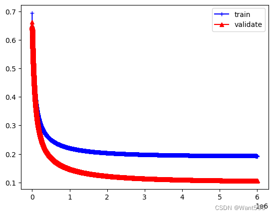
#分析结果,看看在300万轮时的情况
print(cost_lst[500000],cost_val[500000])
0.24994786329203897 0.18926411883434127
#看看5万轮时测试误差
k=50000
w=lst_w[k]
print(cost_lst[k],cost_val[k])
y_p_true=np.array([1 if item>0.5 else 0 for item in h(X_test,w).ravel()])
y_p_true
np.sum(y_p_true==y_test)/X_test.shape[0]
0.45636730725628694 0.45732791872411350.7
#看看8万轮时测试误差
k=80000
w=lst_w[k]
print(cost_lst[k],cost_val[k])
y_p_true=np.array([1 if item>0.5 else 0 for item in h(X_test,w).ravel()])
y_p_true
np.sum(y_p_true==y_test)/X_test.shape[0]
0.40603054170171965 0.394247838217765160.75
#看看10万轮时测试误差
k=100000
print(cost_lst[k],cost_val[k])
w=lst_w[k]
y_p_true=np.array([1 if item>0.5 else 0 for item in h(X_test,w).ravel()])
y_p_true
np.sum(y_p_true==y_test)/X_test.shape[0]
0.381898564816469 0.363559834652638970.8
#分析结果,看看在300万轮时的情况
k=3000000
print(cost_lst[k],cost_val[k])
w=lst_w[k]
y_p_true=np.array([1 if item>0.5 else 0 for item in h(X_test,w).ravel()])
y_p_true
np.sum(y_p_true==y_test)/X_test.shape[0]
0.19780791870188535 0.114326801305738750.85
#分析结果,看看在500万轮时的情况
k=5000000
print(cost_lst[k],cost_val[k])
w=lst_w[k]
y_p_true=np.array([1 if item>0.5 else 0 for item in h(X_test,w).ravel()])
y_p_true
np.sum(y_p_true==y_test)/X_test.shape[0]
0.19393055410160026 0.107541811991899470.85
#在500轮时的情况
k=5999999print(cost_lst[k],cost_val[k])
w=lst_w[k]
y_p_true=np.array([1 if item>0.5 else 0 for item in h(X_test,w).ravel()])
y_p_true
np.sum(y_p_true==y_test)/X_test.shape[0]
0.19319692059853838 0.106027626172624680.85
1.9 如何选择超参数?比如学习率设置多少好?
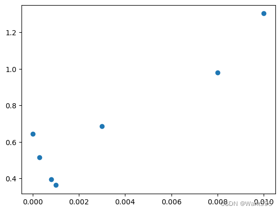
#1 设置一组学习率的初始值,然后绘制出在每个点初的验证误差,选择具有最小验证误差的学习率
alpha_lst=[0.1,0.08,0.03,0.01,0.008,0.003,0.001,0.0008,0.0003,0.00001]
def grandient(X,y,iter_num,alpha):y=y.reshape((X.shape[0],1))w=np.zeros((X.shape[1],1))cost_lst=[]for i in range(iter_num):y_pred=h(X,w)-ytemp=np.zeros((X.shape[1],1))for j in range(X.shape[1]):right=np.multiply(y_pred.ravel(),X[:,j])gradient=1/(X.shape[0])*(np.sum(right))temp[j,0]=w[j,0]-alpha*gradientw=tempcost_lst.append(cost(X,w,y.ravel()))return w,cost_lst
lst_val=[]
iter_num=100000
lst_w=[]
for alpha in alpha_lst:w,cost_lst=grandient(X_train,y_train,iter_num,alpha)lst_w.append(w)lst_val.append(cost(X_val,w,y_val.ravel()))
lst_val
C:\Users\sanly\AppData\Local\Temp\ipykernel_8444\2221512341.py:5: RuntimeWarning: divide by zero encountered in logright=np.multiply(y.ravel(),np.log(y_hat).ravel())+np.multiply((1-y).ravel(),np.log(1-y_hat).ravel())
C:\Users\sanly\AppData\Local\Temp\ipykernel_8444\2221512341.py:5: RuntimeWarning: invalid value encountered in multiplyright=np.multiply(y.ravel(),np.log(y_hat).ravel())+np.multiply((1-y).ravel(),np.log(1-y_hat).ravel())[nan,nan,nan,1.302365681883988,0.9807991089640924,0.6863333276415668,0.3635612014705094,0.3942497801600069,0.5169328809489743,0.6448319202310255]
np.array(lst_val)
array([ nan, nan, nan, 1.30236568, 0.98079911,0.68633333, 0.3635612 , 0.39424978, 0.51693288, 0.64483192])
lst_val[3:]
[1.302365681883988,0.9807991089640924,0.6863333276415668,0.3635612014705094,0.3942497801600069,0.5169328809489743,0.6448319202310255]
np.argmin(np.array(lst_val[3:]))
3
#最好的学习率为
alpha_best=alpha_lst[3+np.argmin(np.array(lst_val[3:]))]
alpha_best
0.001
#可视化各学习率对应的验证误差
plt.scatter(alpha_lst[3:],lst_val[3:])
<matplotlib.collections.PathCollection at 0x1d1d48738b0>
#看看测试集的结果
#取出最好学习率对应的w
w_best=lst_w[3+np.argmin(np.array(lst_val[3:]))]
print(w_best)
y_p_true=np.array([1 if item>0.5 else 0 for item in h(X_test,w_best).ravel()])
y_p_true
np.sum(y_p_true==y_test)/X_test.shape[0]
[[-4.72412058][ 0.0504264 ][ 0.0332232 ]]0.8
#查看其他学习率对应的测试集准确率
for w in lst_w[3:]:y_p_true=np.array([1 if item>0.5 else 0 for item in h(X_test,w).ravel()])print(np.sum(y_p_true==y_test)/X_test.shape[0])
0.75
0.75
0.6
0.8
0.75
0.6
0.55
1.10 如何选择超参数?试试调整l2正则化因子
实验4(2) 完成正则化因子的调参,下面给出了正则化因子lambda的范围,请参照学习率的调参,完成下面代码
# 1正则化的因子的范围可以比学习率略微设置的大一些
lambda_lst=[0.001,0.003,0.008,0.01,0.03,0.08,0.1,0.3,0.8,1,3,10]
# 2 代价函数构造
def cost_reg(X,w,y,lambd):#当X(m,n+1),y(m,),w(n+1,1)y_hat=sigmoid(X@w)right1=np.multiply(y.ravel(),np.log(y_hat).ravel())+np.multiply((1-y).ravel(),np.log(1-y_hat).ravel())right2=(lambd/(2*X.shape[0]))*np.sum(np.power(w[1:,0],2))cost=-np.sum(right1)/X.shape[0]+right2return cost
def grandient_reg(X,w,y,iter_num,alpha,lambd):y=y.reshape((X.shape[0],1))w=np.zeros((X.shape[1],1))cost_lst=[] for i in range(iter_num):y_pred=h(X,w)-ytemp=np.zeros((X.shape[1],1))for j in range(0,X.shape[1]):if j==0:right_0=np.multiply(y_pred.ravel(),X[:,j])gradient_0=1/(X.shape[0])*(np.sum(right_0))temp[j,0]=w[j,0]-alpha*(gradient_0)else:right=np.multiply(y_pred.ravel(),X[:,j])reg=(lambd/X.shape[0])*w[j,0]gradient=1/(X.shape[0])*(np.sum(right))temp[j,0]=w[j,0]-alpha*(gradient+reg) w=tempcost_lst.append(cost_reg(X,w,y,lambd))return w,cost_lst
# 3 调用梯度下降算法用l2正则化
iter_num,alpha=100000,0.001
cost_val=[]
cost_w=[]
for lambd in lambda_lst:w,cost_lst=grandient_reg(X_train,w,y_train,iter_num,alpha,lambd)cost_w.append(w)cost_val.append(cost_reg(X_val,w,y_val,lambd))
cost_val
[0.36356132605416125,0.36356157522133403,0.3635621981384864,0.36356244730503007,0.36356493896065706,0.3635711680214138,0.36357365961439897,0.3635985745598491,0.3636608540941533,0.36368576277656284,0.36393475122711266,0.36480480418120226]
# 4 查找具有最小验证误差的索引,从而求解出最优的lambda值
idex=np.argmin(np.array(cost_val))
print("具有最小验证误差的索引为{}".format(idex))
lamba_best=lambda_lst[idex]
lamba_best
具有最小验证误差的索引为00.001
# 5 计算最好的lambda对应的测试结果
w_best=cost_w[idex]
print(w_best)
y_p_true=np.array([1 if item>0.5 else 0 for item in h(X_test,w_best).ravel()])
y_p_true
np.sum(y_p_true==y_test)/X_test.shape[0]
[[-4.7241201 ][ 0.05042639][ 0.0332232 ]]0.8